Category Archives: Advanced EM

Advanced Electromagentism (Phys 341)

Final Results and Conclusions: Modeling E and B Fields of a Toroidal Conductor to Explore Tokamak Plasmas

I have developed expressions for B, H, and M for the JET tokamak, and have plotted these fields. I began by deriving the expression for the magnetic field of such a system, approximating it as a toroidal solenoid. I followed Griffith’s example 5.10 to arrive at my expression. As mentioned previously, the expression for the magnetic field of this system is:

$\textbf{B(r)} = \frac{\mu_{0} N I}{2 \pi s} \hat{\phi}$.

As mentioned previously, I use the parameter values from the JET project, and will assume that $N = \alpha q(r)$. My first instinct (and the first value of alpha that I tried) was to set $\alpha$ at the circumference of the torus (17.9 m). As will be discussed below, this did not give reasonable results, and I revised the value of alpha accordingly.

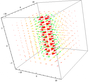
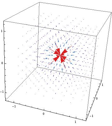
I defined a field (bfield) based on the expression I derived. This was in spherical coordinates since that was easiest to use with the Mathematica command TransformedField. I then transformed this to Cartesian coordinates, and used VectorPlot3D to plot the Cartesian vector field. This produced the circumferential field that I expected. It varies only with distance from the center of the torus ring, and curves around the torus.

The magnetic field, as expected, is purely circumferential and its direction alternates as the current changes. The torus has been superimposed on the field to indicate the region where the field is nonzero.

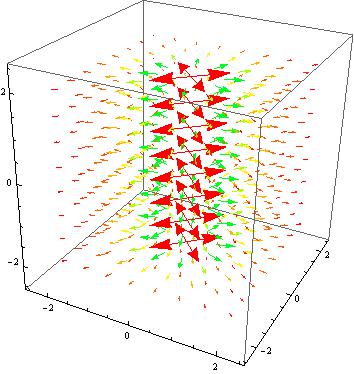
The torus from a different perspective.

I then repeated the same procedure for the Auxiliary field and magnetization, and both produced the fields I expected (both were the same shape but different magnitudes than the magnetic field and the magnetization was in the opposite direction). Magnetization was in the opposite direction of the magnetic field (as expected) because I used the magnetic susceptibility value of hydrogen (since JET used an H or DT plasma) and hydrogen is diamagnetic (as per Griffiths Table 6.1). A tacit assumption here is that this value does not change significantly when the gas is ionized into a plasma. I do not know what effect this would have on my results, but my results should be viewed with this fact in mind.

The Auxiliary field looks very similar to the magnetic field, and, in fact, differs only in that the vectors have different magnitudes.

Note that all of these fields are identically zero for all regions outside of the the volume of the torus. The values described by the vector field only hold for locations where $(R – r/2) \leq s \leq (R + r/2)$. Unfortunately, I was unable to find a way to force Mathematica to either make the vector field zero in this region or two suppress the vectors so that they did not display. Despite this, the field is correct, just over an incorrect range.

The magnetization in the torus, again, has the same shape as the other fields, but opposite sign.

Now, realistically, the current in my expression for these quantities would not be constant, but would vary with time (as tokamaks operate as pulsed, AC devices). This means that $I = I_{0}\cos(\omega t)$. This assumes that that at time zero, the current amplitude is maximum (which is reasonable since the zero point is arbitrary as long as we look at the system sufficiently long after the tokamak operation has begun).

To account for this time dependence, I let $I = I_{0}$ and multiplied in the cosine term. I did this in the VectorPlot3D argument instead of in the definition of my field because the transform would not work with 4 variables. This should not affect the results. I did this for all three fields. As expected, the fields retain their shapes and the vectors alternate direction with current. An example follows, and the rest can be found in the Mathematica notebook:

Magnetic Field Animation

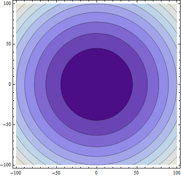
After developing these models, I wanted to use my expression to find the magnetic field at the center of the torus volume. I would then compare this to the established value for JET’s magnetic field, and the difference would speak to the legitimacy of my model and the assumptions I made, specifically the proportionality constant, $\alpha$. The magnitude of the magnetic field as a function is radius was plotted, to emphasize the fact that it varies only with radius and is not constant throughout the torus (since it spans a range of radii).

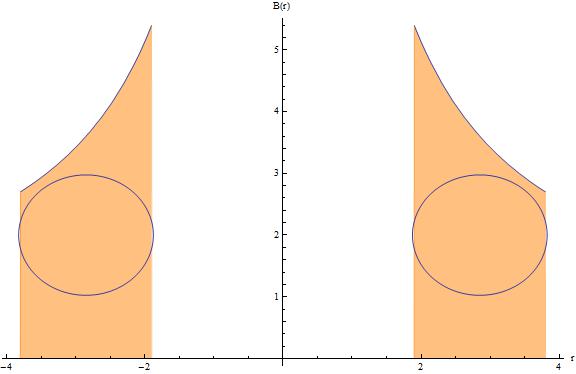
The magnetic field strength as a function of radius, to illustrate the fact that the field is zero outside of the torus and that the field only varies with radius. Note also that it is not constant within the torus, as there are several radii encompassed within it. The surface of the torus is included to illustrate the region with nonzero field.

The magnetic field strength as a function of radius, to illustrate the fact that the field does vary with radius, which is not necessarily clear from the vector fields. . The surface of the torus is included to illustrate the region with nonzero field.

For $\alpha = 17.9$, $B = 22.6$T. The established value is $B = 3.6$T. This is a percent error of over 500%. Since this value of alpha was simply a first guess to see how the model worked, this extremely high percent error should not be alarming. We can easily find a better alpha. Knowing what B should be, and the other constants, we can solve for alpha and get that it should take a value of $\alpha = 2.85$. This is very interesting because this means that $\alpha = R$ and that $N = \alpha q = R q = (2.85)(3) = 8.55$. A value of 8.55 for N means that there are only about 9 windings of the current around the solenoid. In Griffiths’ example, he specifies that we assume the windings to be “uniform and tight enough so that each turn can be considered a closed loop.” 8.55 turns around a circumference of 17.9 meters is probably not sufficiently tight. As such, this model has shown that is model is insufficient to describe the behavior of a tokamak (which is not surprising). As it is, this results indicate our model is imprecise. It also indicates that, perhaps, the current should be modeled as a set of smaller currents with tighter windings superimposed on each other. The next logical step in this research would be to examine what exactly the effects of this fallacious assumption are, and how best to address them.

I would also like to note that, while my original plan was to also model the electric field of this system. In my research I have not found any mention of the electric field of a tokamak reactor, only ever the magnetic field. I assume that this is because the magnetic field is the source of confinement, and thus more interesting. Since the electric field seems to be uninteresting to tokamak research, and since I have nothing against which to compare my model, I will not be modelling this field.

With this model (assuming that the windings were closed loops) changing q had a relatively small effect. According to the expression for magnetic field, changing q changer the magnitude of the field vectors (they are directly proportional). In my Mathematica animations of this, though, the change in vector magnitude was never actually noticeable. As such I conclude that, while the safety factor plays a significant role in tokamak design, due to the simplifications made in my model, it has very little effect.

While my results (that N is small and that q has a negligible effect) both indicate that my model is not sufficiently precise to model a tokamak, this does not indicate failure. The main thing that can be learned from this is that a tokamak’s magnetic field is much more complicated than that of a toroidal solenoid, as the current is at a large angle compared to the plane in which the torus lies as it travels around the torus. While my model is imprecise and does not take this into account, it can produce the appropriate values for magnetic field, but with a compromise.

The assumption that went into my model (Griffiths’) that the current loops were essentially closed meant that we assumed the current had only z an s components (and no phi component). The fact that N is so small relative to the circumference means that the current loops will be more slanted and will have a component in all three directions. Obviously, this means that the expression for magnetic field will be different. In the derivation, the fact that the current had no phi component meant that terms cancelled out, leaving us with a purely circumferential field. Clearly, in an actual tokamak, this is not the case. While it is unfortunate that my results showed my model to be insufficient for a robust model of a tokamak, it has been very valuable in that it has confirmed and emphasized the complexity of a tokamak magnetic system. It also puts the current state of fusion research in a very clear context – research has been going on since the middle of the last century, and yet no viable commercial fusion reactor has been developed. This seems to make sense considering the complexity of the systems.

—

Here is a link to the Mathematica Notebook: https://drive.google.com/file/d/0B-C9MvBAfmyIc01BdHRRbGxoRW8/edit?usp=sharing

Final Data: Diffraction Patterns of C. elegans (revised)

Listed below are five sets of data (3-7), two images each. On the left is the photograph of the fluorescing worm. To the right is its corresponding diffraction pattern, produced with Mathematica.

First, a few comments:

Notice that each worm shape contains a different symmetry (or lack of symmetry). However, every diffraction pattern is symmetrical. The two images tend to share some symmetrical qualities, as noted below each image.

These diffraction patterns are due to the fluorescing parts of the worm (GFP, or green fluorescing protein). I believe that because of my image manipulation (converting to grayscale and brightening the image significantly), the diffraction pattern is approximately due to the entire worm and not just the fluorescing parts.

On that note, I’d like to discuss the parameters I used for image manipulation and Fourier Transforming.

The Fourier Parameters I chose were {0, 1} . These are the default parameters when using the FT command on Mathematica. I chose them among the three most common by ruling out the other two: {-1, 1} is used for data analysis (which I was not doing), and {1, -1} is used for signal processing (also irrelevant to my project). My choice of parameters specified the conventions I wanted the program to use when applying the transform.
The command ImageAdjust [image, {a, b}] adjusts the contrast of the image by a and the brightness by b. For most of my images, I adjusted the contrast by the same amount, but changed the brightness differently for each photo depending on my judgement.
I divided the images by hand and reassembled them according to the image dimensions, rectangles of dimension {col/2, row/2} (where col = the number of pixels in each column of the image, and row = the same for each row). I could have use the command RotateRight, but I did not figure that out until after I developed this equally effective algorithm.

IMAGE 3

This image has axial symmetry perpendicular to the axial symmetry of the worm. The worm is mostly linear, and so is the diffraction.

(complete file for image 3: book 3 )

IMAGE 4

See comment for image 3.

(complete file for image 4: book 4 )

IMAGE 5

Although this does not have an “inversion center” (the worm does not complete a loop), it is significantly less straight than the first few examples. Correspondingly, the diffraction pattern has an axial symmetry perpendicular to the “axis” of the worm. However, it splays out to a higher degree, indicating that the area of the pattern corresponds with the curvature of the worm.

(full file for image 5: book 5 )

IMAGE 6

This further backs up my hypothesis from image 5. The curvature of the worm is great and the area of the pattern is also large. However, this worm does have a sort of “inversion center.” The diffraction image has an eye in the center, which is different than all of the preceding images. The curvature of the worm greatly effects the produced image, which is not surprising, but the overall shape of the image changes dramatically. With more circular worms, an “eye” is formed in the center of the diffraction pattern, and the pattern here has both some rotational symmetry and axial symmetry. With straighter worms, the diffraction is much more linear, containing only axial symmetry.

(full file for image 6: book 6 )

IMAGE 7

See comment for image 6.

(full file for image 7: book 7 )

Project Plan

Measuring and Modeling Physical RCL Circuits

Purpose and Goals:

The purpose of this project is to demonstrate the difference between theoretical descriptions/relationships of basic LC circuits and experimental values. This is also an exercise in developing a deeper understanding of the theoretical equations governing these relationships. I will record the voltage drop across various components in each circuit and plot them in comparison to the theoretically predicted values. In addition, I will try to answer questions such as “What are the probable causes for deviation from predicted values?”

The first and most simple circuit I will work with is a basic LC circuit:

The DC power source charges the capacitor until it is discharged (via switch) into the right hand circuit. In theory the current should oscillate back and forth between the capacitor and inductor indefinitely if there was no resistance in the circuit. Actual experimental measurements should reveal some resistance due to the wires and components themselves. Below is the start of my derivations for the voltage across each components:

Kirchoff’s Loop Law states that the total voltage drop across the right hand circuit loop should be zero:

$\Delta V_{L}+\Delta V_{C}=0$ (1)

We know that the voltage drop across an inductor is equal to L(dI/dt) and across a capacitor is Q/C:

$L\dfrac {d^{2}Q\left( t\right) } {dt^{2}}+\dfrac {Q\left( t\right) } {c}=0$ (2)

Which can be rewritten as

$\dfrac {d^{2}Q\left( t\right) } {dt^{2}}+\omega _{0}^{2}Q\left( t\right) =0$ (3)

Leaving us with the general solution to this second order differential equation

$Q\left( t\right) =Q_{0}\cos \left( \omega _{0}t-\delta \right)$ (4)

The derivation of the above equations will be more thorough in future posts.

RLC circuit

This circuit is dampened with a resistor, and thus no longer resembles simple harmonic motion, but rather a damped harmonic oscillator.

Kirchoff’s Loop Law now reads

$\Delta V_{L}+\Delta V_{R}+\Delta V_{C}=0$ (5)

$L\dfrac {dI} {dt}+RI +\dfrac {Q} {C} =0$ (6)

Which leaves us with a new second order differential equation

$L\dfrac {d^{2}Q\left( t\right) } {dt^{2}}+R\dfrac {dQ\left( t\right) } {dt}+\dfrac {Q\left( t\right) } {c}=0$ (7)

$\dfrac {d^{2}Q\left( t\right) } {dt^{2}}+\dfrac {R} {L}\dfrac {dQ\left( t\right) } {dt}+\dfrac {1} {LC}Q\left( t\right) =0$ (8)

$\dfrac {1} {LC}\equiv \omega _{0}^{2}$ (9)

$\dfrac {R} {L}\equiv 2\beta$ (10)

$\dfrac {d^{2}Q\left( t\right) } {dt^{2}}+2\beta \dfrac {dQ\left( t\right) } {dt}+\omega _{0}^{2}Q\left( t\right) =0$ (11)

Eq. (11) is the second order differential equation governing the charge on the capacitor as a function of time and thus describing the voltage drop and current through the other components of the circuit.

Predictions

Theoretically I should expect the voltage across the components in an LC circuit to oscillate indefinitely according to simple harmonic motion. I expect that with a real circuit this would not be the case. A physical LC circuit would actually behave as if a resistor was in series with the two components, causing the amplitude of the oscillations to decrease over time. This is because the circuit parts, such as the wires connecting each component, are not ideal and have resistance.

I predict that a graph of the voltage difference over time for a given component will appear as a decaying sinusoidal wave. In other words it should resemble an dampled oscillation.

Methods

I will use a PicoScope digital oscilloscope to measure the voltage difference across the capacitor in the LC circuit. In this way I will both be able to see the voltage the capacitor is initially charged to as well as record the transition from a steady voltage to an oscillating voltage.

Sources, Resources, and Parts Needed

Equipment Needed:

DC power source, AC frequency generator, Oscilloscope, Computer, Multimeter

Parts Needed:

Breadboard; various values of resistors, capacitors, and inductors; switch; wires/alligator clips

Helpful Texts:

Physics for Scientists and Engineers: A Strategic Approach with Modern Physics (2nd ed.) by Randall D. Knight
Introduction to Electrodynamics (4th ed.) by David Griffiths
Data Reduction and Error Analysis for the Physical Sciences by Philip R. Bevington, D. Keith Robinson
Experimentation : an introduction to measurement theory and experiment design by D.C. Baird
Ordinary Differential Equations by Morris Tenenbaum and Harry Pollard
Class notes – Classical Mechanics (PHYS 210), Zosia Krusberg.

Websites:

http://www.digikey.com/schemeit (for creating circuit schematics)

Timeline

Week 1 – April 20th-26th. Acquire all equipment and parts needed for experiment: Talk to Larry Doe for parts and possibly a power source. Talk to David Rishell about an AC signal generator. Setup experiment in Mudd 216 with Prof. Magnes’ oscilloscope, DC power source, and multimeter.

Week 2 – April 27th-May 3rd. Derive equations to predict voltage drop across components to plot on top of collected data. Those equations being ΔV for LC, dampened LC (RLC), and AC driven RLC in series circuit. Collect data on voltage drops across LC and dampened LC circuit components. Plot data in mathematica.

Week 3 – May 4th-10th. Collect data on voltage drops over AC driven circuit. Predict resonance frequency. Define equations governing resonance frequency and find actual resonance frequency of circuit. Plot findings in mathematica. Consider sources of error or causes of deviation from predicted values on all three circuit configurations.

Week 4 – May 11th-17th. Finish data collection and additional exploration/inquiry. Create time dependent plots in mathematica to demonstrate projected vs experimental values.

Place/Logistics

Experimentation and data collection will occur in Professor Magnes’ lab in Mudd 216. Brian and Tewa generally work MWF and can be contacted for access to the lab.

Preliminary Data: Magnetic Field Modeling

In this post I will describing the specific charge distributions that I will be modeling and showing a brief derivation for the formulas I calculated.

Cylinder:

Problem 5.14 of Griffiths’ Introduction to Electrodynamics 4th edition describes a long cylindrical wire of radius a and steady uniform flowing current I over the outside surface of the cylinder. The magnetic field outside of the wire can be easily found by using Ampere’s Law.

$\oint \mathbf{B}\cdot dl=\mathbf{B}\oint dl=\mathbf{B}2\pi s=\mu_{0}I_{enc}=\mu_{0}I$

(1) $\begin{equation*} \mathbf{B}(s)=\frac{\mu_{0}I}{2\pi s}\widehat\theta& : s > a \end{equation*}$

When looking at points inside of the cylinder, or $s<a$ , $I_{enc}=0$ and so we know that:

(2) $\begin{equation*} \mathbf{B}(s)=0& : s < a \end{equation*}$

Combining our two cases in (1) and (2) we have:

(3) $\begin{equation*} \mathbf{B}(s) = \left\{ \begin{array}{lr} \frac{\mu_{0}I}{2\pi s}\widehat\theta & : s > a\\ 0 & : s < a \end{array} \right. \end{equation*}$

This is plotted below using Mathematica.

Cylinder

As expected, the magnetic field follows the commonly known right-hand-rule where the direction of the current curls around the direction of current.

Plane -> Slab :

Problem 5.15 of Griffiths’ Introduction to Electrodynamics 4th edition, a thick infinite slab extending from z=-a to z=a carries a uniform volume current $\mathbf{J}=J\widehat x$ . The magnetic field inside of the slab can found using Ampere’s Law again.

$\oint \mathbf{B}\cdot dl=\mathbf{B}\oint dl=\mathbf{B}l=\mu_{0}I_{enc}=\mu_{0}IzJ$

(4) $\begin{equation*} \mathbf{B} = -\mu_{0}Jz\widehat y & : -a > z > a \end{equation*}$

When looking at point outside of the slab, our $I_{enc}=\mu_{0}IaJ$ , and so,

(5) $\begin{equation*} \mathbf{B} = \left\{ \begin{array}{lr} -\mu_{0}Ja\widehat y & : z > a\\ \mu_{0}Ja\widehat y & : z > -a \end{array} \right. \end{equation*}$

Sphere -> Ring:

After some research and individual work, I have come to realize that the magnetic field of either rotating conducting sphere or a spherical solenoid is very complicated. I decided to simplify the distribution to two dimensions rather than three for now. A sphere can be viewed as a collection of disks or rings, so I derived the formula for the magnetic field of a ring with radius R and steady current I .

By setting our coordinate system at the center of the ring, we know that the horizontal components of the magnetic field will cancel out through symmetry and the principle of superposition, and we are left with only the vertical component. This leaves us with:

$\mathbf{B(z)} = \frac{\mu_{0}I}{4\pi}\int \frac{dl}{\mathbf{r}^2}cos\theta$

where $\theta$ is defined as the angle between the wire and our position vector $\mathbf{r}$ . It follows then that

(6) $\begin{equation*} \mathbf{B(z)}=\frac{\mu_{0}I}{2}\frac{R^2}{(R^2+z^2)^{3/2}} \end{equation*}$

References:

Griffiths’ Introduction to Electrodynamics 4th edition

Mathematica Notebook:
https://drive.google.com/file/d/0B4ANWxS26h4FRE53d0d5aFRaN0U/edit?usp=sharing

Preliminary Data

The first item to be modeled will be the electric field of a sphere of uniform charge density. This will set the basic framework for any fields based off of a sphere.

To start, imagine a conducting solid sphere of some radius “R” that contains a total charge of Q. There are a couple of ways that the electric field of this configuration could be found. One is Coulomb’s Law, given by:

$E(r)= \frac{1}{4\pi\epsilon_0} \int {\frac{\textbf{$\hat{r}$}}{r^2} dq$

Where $ \epsilon_0 $ is the permittivity of free space and $ r $ is the separation between the source and the test.

The other (and far easier) is to use Gauss’s Law, given by:

$\oint _S {\textbf{E} \cdot d\textbf {a} = \frac{1}{\epsilon_0} q_e$

Where $q_e$ is the enclosed charge of a Gaussian surface, $\textbf{E}$ is the electric field. Note that we are also taking a surface integral. All the math looks interesting, but what is a Gaussian surface? A Gaussian surface is an arbitrary surface at some distance from our actual surface (in this case our actual surface is the previously mentioned sphere), that matches the symmetry of the electric field generated by the object in question. What that means is that the electric field of our real object “flows” through the Gaussian surface in the same way it does the real object. Once this surface has been drawn we can use Gauss’s law to solve for the electric field of the object. In our case, the Gaussian surface is a sphere around out real sphere of some radius that is greater than $R$.

Now, because of symmetry, we can make a few nice simplifications. First, since the magnitude of the electric field is constant (the sphere is uniformly charged) $\textbf{E}$ can be taken outside of the integral, leaving the only thing inside to be $d\textbf {a}$. The integral of that is simply “A” but recall that this was a surface integral, so A is the surface area of our Gaussian surface, a sphere, which is simply $4 \pi r^2$.

Now all we have left is

$\textbf{E}\ (4 \pi r^2) = \frac{1}{\epsilon_0} q_e$

Which is easily re-written as

$\textbf{E} = \frac{q_e}{\epsilon_0 4 \pi r^2} \textbf{$\hat{r}$}$

and there is it. The electric field of a sphere (Griffith’s Example 2.2).

The electric field plotted 3D in mathematica:

Next, we’ll find the electric field of a cylinder of length L and radius R with a uniform volume charge density $\rho$. Again, it will be quite a bit easier to determine this using Gauss’s Law:

$\oint _S {\textbf{E} \cdot d\textbf {a} = \frac{1}{\epsilon_0} q_e$

Just like the sphere we draw a surface that matches the symmetry of our object, and since we want the field outside the cylinder, we again choose a surface that has a radius greater than R, which I’ll call r.

Following the same line of reasoning as the sphere, the left side of the equation can be simplified to just the electric field, E, multiplied by the surface area of the surface. The surface area of a cylinder is given by $2\pi r l$ where $l$ is just the length of of Gaussian cylinder. This lets us write:

$\textbf{E}\ (2 \pi r l) = \frac{1}{\epsilon_0} q_e$

From here we need to find a way to express our charge enclosed. The definition of volume charge density is the total charge over the total volume, meaning that total charge is equal to charge density multiplied by the volume of the object. Again call our total charge Q and we know the volume of a cylinder to be $\pi r^2 l$. Taking our radius as R we can now write our Gauss’s law expression as:

$\textbf{E}\ (2 \pi r l) = \frac{\rho\ \pi R^2 l}{\epsilon_0}$

Solving for $\textbf{E}$ yields:

$\textbf{E} = \frac{\rho R^2 }{2r\epsilon_0} \textbf{$\hat{r}$}$

Which is nicely plotted as:

(excerpt from Griffith’s problem 2.16)

Finally, we have the electric field of a bar. The electric field analogue to a bar magnet is whats known as a bar electret. For this type of model, we will assume that the electret’s shape is similar to the more common picture of a bar – that is that it’s length is much greater than its width.

This electret requires us to use something other than Gauss’s Law. In this configuration the electric field is approximately that of two point charges of opposite charge. The electric field of a point charge is given by:

$\textbf{E} = \frac{q}{\epsilon_0 4 \pi r^2} \textbf{$\hat{r}$}$

The plots shown below are of the two points of opposite charge.

and

The mathematica code for these figures may be viewed here: Preliminary Data

Further modeling may show more complex systems build off of the ones shown here.

Railgun Physics Preliminary Data: Derivations and Realizations

The brunt of my Mathematica work thus far can be found here: https://drive.google.com/file/d/0B0sdNVAIz9CjZkpLbnJEbTZjYXM/edit?usp=sharing

A rail gun is a simple assembly involving more complicated physics. It consists of a power supply connected to two parallel rails. Between these rails is a projectile that completes the circuit. The power supply (in this case we are modeling it as several capacitors) will release current into the circuit, instigating a number of forces which we will attempt to model. Below is a very generic

railgun

example of a rail gun circuit. Our original goal was to find the equations of motion for the railgun and hence functions for velocity and position. However, the mathematics required for this project has revealed itself to be immensely complicated, certainly much more so than we had expected. Many of the preliminary equations we find are based on the velocity itself, something we cannot know until the very end under our current plan. We have decided to go about it a different way, solving for all the relevant phenomena we had previously sought (current, b-field, emf) and using standard speeds of rail guns as constants to model said phenomena. In both our projects we will begin by deriving the most generic version of the magnetic field, caused by some current flowing through the circuit. This will require the Biot-Savart law:

(1) $\begin{equation*} B=\frac{\left(\mu _0I(t)\right)}{4\pi }\int \frac{dl\times r}{r^2}\) \end{equation*}$

From Griffiths, the magnetic field at a point near a current carrying wire will be:

(2) $\begin{equation*} B=\frac{\left(\mu _0I\right)}{4\text{$\pi $z}}*\left(\sin \left(\theta _1\right)-\sin \left(\theta _2\right)\right) \end{equation*}$

Here, the magnetic field at a point p is a superposition of the magnetic fields created by the four sections of the current carrying wire. B1 and B3 will be the fields of the two rails, B2 will be the field of the projectile, and B4 will be the field of the power source.

(3) $\begin{equation*} B_1=\frac{\mu _0I}{4\pi }\left(\frac{1}{y}\left(\frac{x}{\sqrt{x^2+y^2}}-\frac{(L-x)}{\sqrt{(L-x)^2+y^2}}\right)\right) \end{equation*}$

(4) $\begin{equation*} B_2=\frac{\mu _0I}{4\pi }\left(\frac{1}{(L-x)}\left(\frac{y}{\sqrt{(L-x)^2+y^2}}-\frac{(d-y)}{\sqrt{(L-x)^2+(d-y)^2}}\right)\right) \end{equation*}$

(5) $\begin{equation*} B_3=\frac{\mu _0I}{4\pi }\left(\frac{1}{(d-y)}\left(\frac{(L-x)}{\sqrt{(L-x)^2+(d-y)^2}}-\frac{x}{\sqrt{x^2+(d-y)^2}}\right)\right) \end{equation*}$

(6) $\begin{equation*} B_4=\frac{\mu _0I}{4\pi }\left(\frac{1}{x}\left(\frac{(d-y)}{\sqrt{x^2+(d-y)^2}}-\frac{y}{\sqrt{x^2+y^2}}\right)\right) \end{equation*}$

The total field, of course, would be the superposition of these four equations. However, after having done a good amount of research and going through trial and error, we have discovered that when the rails (L) are much longer than the projectile and power source (d), we only need include the effects of the rails. Below is this magnetic field:

(7) $\begin{equation*} B_{\text{tot}}=\frac{\mu _0I}{4\pi }\left(\left(\frac{1}{y}\left(\frac{x}{\sqrt{x^2+y^2}}-\frac{(L-x)}{\sqrt{(L-x)^2+y^2}}\right)\right)+\left(\frac{1}{(d-y)}\left(\frac{(L-x)}{\sqrt{(L-x)^2+(d-y)^2}}-\frac{x}{\sqrt{x^2+(d-y)^2}}\right)\right)\right) \end{equation*}$

Now, to find the magnetic field upon the projectile itself, we substitute L for x and get:

(8) $\begin{equation*} B_{\text{proj}}=\frac{i \mu _0 \left(\frac{L}{y \sqrt{L^2+y^2}}-\frac{L}{(d-y) \sqrt{(d-y)^2+L^2}}\right)}{4 \pi } \end{equation*}$

From here, it is my responsibility to find out how the rail gun acts as a circuit. There are a couple parameters that I have been able to establish pretty easily. The first is the resistance of the circuit as a whole. This resistance is:

(9) $\begin{equation*} R=\rho \frac{(2L+2d)}{A} \end{equation*}$

Where \rho is the resistivity and A is cross sectional area.

From there, we can start to look at the current created by the a capacitor with charge Q_0 and capacitance C discharging with the generic

(10) $\begin{equation*} I_{\text{cap}}=\frac{Q_0}{\text{RC}} \end{equation*}$

By replacing the R term we found above,

(11) $\begin{equation*} I_{\text{discharge}}=\frac{Q_0}{\text{C$\rho $}\frac{(2L+2d)}{A}}e^{\frac{-t}{\rho \frac{(2L+2d)}{A}C}} \end{equation*}$

We also know that this current is not the only current present in the circuit, as there is an induced current caused by the EMF created by the changing area and Magnetic Field (aka Magnetic Flux). We know that EMF ( \epsilon ) is equal to:

(12) $\begin{equation*} -\frac{\text{d$\phi $}}{\text{dt}}=\frac{\text{dB}}{\text{dt}}d\frac{(\text{dx})}{\text{dt}} \end{equation*}$

We use the chain rule to say that:

(13) $\begin{equation*} \frac{\text{dB}}{\text{dt}}=\frac{\text{dB}}{\text{dL}}\frac{\text{dL}}{\text{dt}\\ } \end{equation*}$

Where the second term

(14) $\begin{equation*} \frac{\text{dL}}{\text{dt}}=v \end{equation*}$

Solving for the derivative of B with respect to L, I got that

(15) $\begin{equation*} \frac{\text{dB}}{\text{dL}}=\frac{i \mu _0 \left(\frac{\frac{1}{\sqrt{(d-y)^2+(L-x)^2}}-\frac{(L-x)^2}{\left((d-y)^2+(L-x)^2\right)^{3/2}}}{d-y}+\frac{\frac{(L-x)^2}{\left((L-x)^2+y^2\right)^{3/2}}-\frac{1}{\sqrt{(L-x)^2+y^2}}}{y}\right)}{4 \pi } \end{equation*}$

It is after this step where it gets complicated. I have used this expression to solve for EMF and then current, but the results are far from elegant and I am going to withhold them until I can validate the methodology. From here, there are two options. Griffiths proposes that EMF simply equals this result times velocity. However, I think that I may have to integrate the magnetic field over the area of the loop. I have tried this and have not had luck; the integral has been equal to 0 every time I’ve tried, something I know to be false. Once I figure this out, I will be able to animate and model all of these expression, and collaborate with John to achieve our final result.

As for our physical model, we will work with Professor Magnes to find something safer and more practical in the context of Vassar.

References:

Griffiths, David J. Introduction to Electrodynamics. Upper Saddle River, NJ: Prentice Hall, 1999. Print.

http://webphysics.davidson.edu/physlet_resources/bu_semester2/c11_RC.html

https://physics.le.ac.uk/journals/index.php/pst/article/viewFile/468/275

Preliminary Data, Magnetic Fields and force in a railgun

From Biot-Savart law of a wire in a closed loop can be broken into 4 parts. Additionally, it should be noted that when considering Ampere’s Law:

The displacement current term is expected to be negligible. That is because in order for the instantaneous rate of change of the electrical field to be significant, the power, loop size and switching rate would have to be extremely, large, small and fast, respectively. Furthermore, for a railgun that size, the current term dwarfs the displacement term by several magnitudes, rendering it irrelevant.

Where z is the shortest distance from a point in space to the wire and theta and phi are the angles between the beginning and end of the wire, respectively. Modeling the circuit as four line currents then allows us to break the B field into four components and solve the above equation, yielding:

railgun

It should be noted that L is the distance from the start of the rail to the slug and is time dependent, x is the distance along the rails, d is the separation between the rails and y is the distance from the bottom rail. Combining these terms using the law of superposition gives the total magnetic field at any point within the loop.

Capture

However, since we are interested in the magnetic field on points within the slug, however, we can set x=L and remove the Bback and Bslug term. The removal of these terms originates from the fact that the nonrail sections are far removed from the slug and generate no significant field within the loop. Additionally, the Bslug term can be removed since due to conservation of momentum, the external magnetic field upon the slug can not be generated by the slug. Additionally, in order to ease calculation, we assume the slug is thin in the x direction, so that we do not have to include width considerations in our calculations. Therefore the Magnetic field upon a point within the the slug (hereafter referred to as B) is:

Next, we will calculate the force upon the slug. Using the Lorentz force law, F=I(dlxB). Since railguns are extremely high energy devices, using enormous currents withing the rails while firing, the best way to power these devices is using capacitors. As a result, the current is variable with time as the capacitor discharges. Additionally, as a result of Faraday’s law, there is an emf generated in the loop as the current and loop size vary, which also affects the current as a function of time.

The force direction is determined by the right hand rule between the direction of the current and the B field within the slug. For a counter clockwise current, the current flows in the positive y direction and the B field for all wire components, including the back and slug, point in the positive z direction (out of the page in the diagram), giving a right hand rule direction of +x.

Additionally, the B field described above is for a specific location along the projectile, and as such the B field must be integrated over the width of the slug. The total magnetic force on the slug therefore becomes:

The magnetic force can also be used in Newton’s Second law to solve for the current in the slug. Of course, this is entirely inaccurate, as there are several means for the current to change, including thermal radiation, rotation and voltage gaps between the slug and the rails. These effects are difficult to calculate and not the subject of this project, suffice to say that the most common method of dealing with these forces is to see what portion of the force is lost.

Since L is time dependent, and extremely fluid, the most common way of reducing this equation is to take the spatial terms and group them into a quantity called the inductance gradient. This quantity is the result of the complex induction effects within the circuit, and is dependent upon the waveform of current, geometry of rails, materials of rails and projectile This quantity, however, cannot be determined theoretically. There are not enough governing equations to solve for L. Instead, what papers concerning railguns use are complicated regression models to determine the optimum dimensions for the rails to maximize this inductance gradient, some of which will be modeled using mathematica in the final data. Therefore, the instantaneous force on the slug can be modeled as:

The Current, being modeled by Elias Kim, can then be inserted into this equation to provide an instantaneous force upon the projectile as a function of t, which can the be solved to (hopefully) provide equations of motion for the slug, and at the very least provide a unsolvable differential equation.

In this reduced form, it becomes clear that the most important factor in this equation is the current, which exponentially increases power as it is made bigger. The 1/2 scalar multiple is the result of the common approximation that half of the current in the loop is required to maintain the expanding magnetic fields, and that only the other half produces force. The navy recently tested a gun that fired a 3.2kg slug over mach 7, this gun used over 33MJ of energy.

As for our physical construction, we had some “technical” difficulties with our design and the small issue of it firing a lethal projectile with highly expensive, dangerous materials. As such we are currently working to scale down our design and will construct it and test this weekend, posting the final specifications and results during the final data.

Mathematica Notebook: https://drive.google.com/a/vassar.edu/?tab=mo#folders/0B0K4JjJfDy1fNnE4MHJON0k4TDg

References:

http://web.mit.edu/mouser/www/railgun/physics.html

Elias Kim

http://ikiu.ac.ir/public_files/profiles/items/1295865343.pdf

http://www.livescience.com/7463-navy-tests-incredible-sci-fi-weapon.html

Preliminary Data: Capacitors

Summary of Progress up to this Point:

I have found the energy storage capability of a simple, slightly physically impractical, square parallel plate capacitor. Compared to the idealized model taught in introductory physics, this capacitor stores 94.34% the energy, the discrepancy likely caused by the finite dimensions of the plates. The accuracy of my model is likely high based on a comparison of the methods used and a sampling of values produced by the exact, theoretical model.

Details:

Recall Coulomb’s Law for a charged surface: $\vec{E}(\vec{r}) =\frac{1}{4 \pi \epsilon_0} \int \frac{\sigma\left(\vec{r'}\right)}{\mathfrak{r}^{2}}\hat{\mathfrak{r}} \: da'$ . In Cartesian coordinates for a flat plate lying in the xy-plane at z=0, this can be more explicitly written as:

$\vec{E}(x,y,z)=\frac{1}{4 \pi \epsilon_0}\int_{y'_i}^{y'_f}\int_{x'_i}^{x'_f}\sigma\frac{(x - x', y - y', z - z')}{((x - x')^2 + (y - y')^2 + (z - z')^2)^{3/2}}\mathrm{d}x'\mathrm{d}y'$

This complicated multi-variable vector integral expression is actually executed correctly by Mathematica, giving the field at a point very close to the middle of a rectangular charged plate, or of any point fairly far away from the plate in a short time (~10 seconds at the most on my personal computer). However, at points very close to the plate at an arbitrary location (for example, half-way between the center and a corner) the program took several minutes to evaluate; not a practical outcome. Therefore, my method of splitting the plane into thousands of tiny point charges (which is computationally efficient everywhere) needed to be examined for accuracy.

This method is built on the simpler form of Coulomb’s Law for a point charge: $\vec{E}(\vec{r})=\frac{1}{4 \pi \epsilon_0}\frac{q}{r^2}\hat{r}$ but is applied across thousands of point charges that form a grid superimposed over the plane being studied (the limit as the number of tiny charges approaches infinity is the exact expression). This method is extremely accurate at a distance, but up close it breaks down as the quantization of charge is noticeable, unfortunate given that capacitors are being studied. Therefore, the field produced by two slightly different arrangements was examined. For example, a grid of 100×100 points was calculated and averaged with a field produced by a 101×101 grid. This was done because a point that is very near a charge for one configuration is commensurable far away from the nearest charges for the other configuration. Averaging these out produces a value very close (only 0.04% too high) to the field of the theoretical model.

Once the model was justified, the points being tested were selected. Only points half-way between plates were evaluated because getting to close to the grid resulted in inaccurate values for the E-field, despite the otherwise successful attempt above to “smooth out” the point charges. Sampling this narrow range was justified because the exact method showed that the field varies by less than a percent across the small separation gap between plates. The values for the charge placed on the plates was taken from a problem in Knight.

To save time for the heavy computation, symmetry was invoked. Recognizing that only one quadrant of the area between plates needed to be evaluated, and that only one plate needed to be examined (because plates are identical aside from their charge sign), the computation was performed in one eighth the time previously expected. Nevertheless, the computation of the electric field at 256 points close to the plate took 10 minutes and 18 seconds when run through the relatively fast and efficient servers available to Vassar students through VApps.

To find the energy stored within, I had to reverse engineer eq. 2.45 (Griffiths, 4th Ed.). Instead of using the integral that describes the energy in a capacitor $W=\frac{\epsilon_0}{2}\int E^2 (\vec{r})\mathrm{d}\tau$ , I instead broke this integral into a sum:

$W=\frac{\epsilon_0}{2}\sum_{i}E^2 (\vec{r}_i)\Delta V$

where ΔV was the area in the immediate vicinity of the point sampled (for all 1024 of the evenly-spaced points, this was simply 1/1024 the total volume). This was necessary because I only have a quantized set of point at which I know the electric field, rather than an integrable function for the electric field.

In summary for the data gathered thus far, the energy stored in a 2 meter by 2 meter parallel plate capacitor with a separation of 2 centimeters is 0.2664 mJ. The basic approximation, where $\vec{E}_{ppc}=\frac{\sigma}{\epsilon_0}\hat{n}$ , resulted in 0.2824 mJ.

Next Steps:

As of yet, no visual aids have been developed due to the numerical nature of the early stages of the project. As the first heavy computation has been done and shown to be a success, time can now be devoted to the following:

Illustrating the fringing field at the very edge of a capacitor. This is likely one of the causes of the reduced energy storage observed compared to the infinite approximation, thus it would be an important concept to visualize.
Running a few more capacitor simulations and plotting the effect of plate separation on energy storage.

The math behind calculating related values (such as capacitance or the effect of an added dielectric) is fairly straightforward and can be saved until the end.

References:

Griffiths, Electrodynamics 4th Ed.
Knight, Physics for Scientists and Engineers 2nd Ed

Mathematica:

Main File: https://www.dropbox.com/s/2ab6445v9s95xvz/ModelingCapacitors_Kachelein_PHYS341_2014.nb
Data File: https://www.dropbox.com/s/47apmk39swj0ucn/ModelingCapacitors_Kachelein_PHYS341_2014_GIANT%20DATA%20FOLDER.nb

Preliminary Results: Mie Scattering and the Interstellar Medium (ISM)

Reflections

An important question emerges in the study of scattered light in the interstellar medium (ISM). Why use the Mie solutions to Maxwell’s equations as opposed to the Rayleigh or Debye methods for modeling this scattering? As with many other methodological decisions, the answer lies in the physical parameters and observational requirements of the system that I’m trying to model. Optical observational data of extinction due to dust grains as a function of wavelength is denoted by: $A_\lambda$ and this observed data necessitates that the extinction be inversely proportional to wavelength:

$A_\lambda\propto\lambda{^-1}$

i.e. the wavelength must be approximately the size of the grains in question. Only with that dependency will the the model fit the data. Wavelength dependencies for Rayleigh and Debye scattering do not provide the necessary proportion.

Asymmetry parameter, g

Modeling the Mie solutions to Maxwell’s equations for scattered light by spherical particles has proven tricky. My attempts so far at getting my Mathematica code to work have hit a bit of a snag, with a plot of the asymmetry parameter, g, versus grain size getting stuck on execution of the code (“running”). I am looking into the possibility that I am unable to execute code due to my laptop’s computational strength – a factor that I entirely did not rule into my planning when I laid out my timeline for the project.

Below I’ve laid out my own navigations through Mathematica 9 and the ongoing process of modeling. I made some simplifying (and yet physically relevant) assumptions. The spherical grains will be water ice with an index of refraction of n=1.33. The vacuum will have an index of refraction of n=1. Items [k, 1] and [k, 2] are coefficients for the imaginary portion of the indices of refraction. I have assumed a wavelength within the optical spectrum. [K, 1] – [K, 3] are the wave numbers for the different indices and included are the wavelengths necessary to derive those wave numbers. Lastly I have provided an arbitrary, placeholder grain radius.

I have also defined grain size parameters, necessary for the calculation of the coefficients $a_n$ and $b_n$, shown below.

Part of the complexity and my uncertainty in my code comes in trying to define a complex conjugate function used in the derivation of the Ricati-Bessel and Bessel functions. Below I’ve included the complex conjugate function that I’ve been utilizing.

Helpfully, Mathematica has Bessel functions built in, what I’ve attempted with them is listed below. Note that I am using density as a means of utilizing the Ricati-Bessel functions (wave functions) on a spherical grain. Depending on an interstellar grains properties, i.e. if it’s dielectric and thus has a real index of refraction or it has a complex index of refraction (impure water ice grain), the Bessel or Ricati-Bessel function will change.

Lastly, here’s my code for the coefficients, $a_n$ and $b_n$. $\alpha$ and $\beta$ have been replaced with q, but those values are still the size parameters.

On a side note, this snag has altered my perspective on the nature of computational modeling. I better appreciate the power and growing accessibility to supercomputing.

Resources

Introduction to Electrodynamics, 4th ed. by David J. Griffiths
Physics of the Galaxy and Interstellar Matter by H. Scheffler and H. Elsässer
Interstellar Grains by N.C. Wickramasinghe
Physical Processes in the Interstellar Medium by Lyman Spitzer, Jr.
The scattering of light, and other electromagnetic radiation by Milton Kerker
Mathematica 9 Help Documentation Center (the most valuable resource!)

Mathematica notebook: https://drive.google.com/file/d/0B_r-c0PTUHZldHVNREtrWHlzZXc/edit?usp=sharing

Final Submission

https://vspace.vassar.edu/kaspuhler/projectEM.nb

Two of the best known areas of physics are Maxwell’s classical formulation of electromagnetism and Einstein’s special theory of relativity. The former explains the motion of charged bodies moving at negligible fractions of the speed of light over distances sufficiently large that quantum behavior can be ignored while the latter allows one to analyze the motion of bodies moving at speeds comparable to those of the speed of light. These are standard lenses of consideration that are familiar to any physics student. What is perhaps unknown to many undergraduate students is the deep connection between classical electromagnetism and special relativity. Maxwell’s formulation was the primary development that allowed Albert Einstein to develop a relativistic geometry of the electromagnetic field, Einstein’s work then flowed back in the opposite direction and many of the principles of relativity now form a backbone in modern reformulations of electrodynamics.

The connection between the two fields is made evident by the very title of Einstein’s first paper introducing relativity, “On the electrodynamics of moving bodies.” The paper opens with a discussion of a conductor moving through the field of magnet with velocity $\vec{v}$, as illustrated below:

Assuming the general trend that Galileo discovered—that the laws of physics were the same in all inertial frames of reference—continued to hold true in 19th century physics, Einstein figured that the physics one observers in this configuration should be independent of whether we take the magnet to be at rest or the conductor to be at rest in the same way that the physics of two equally sized bodies colliding, each with velocity $\vec{u}$, is the same as the physics of one of those bodies travelling with velocity $2\vec{u}$ hitting the other body at rest (or more generally, the two objects colliding with any two velocities $\vec{u_a}$ and $\vec{u_b}$ such that $\vec{u_a}+\vec{u_b}=2\vec{u}$). As Einstein notes however this is not the case and the mechanics of the problem are asymmetric, Maxwell left us at a point where choosing a rest frame to solve this problem in requires us to realize one of two asymmetric situations, one in which the force on the conductor comes from a classical electric field and another where the force on the conductor arises from an independent magnetic field.

We examine both reference frames. First consider the rest frame of the magnet, in which there is a static magnetic field $\vec B(\vec r)$ and the conductor approaches the stationary magnet with some velocity $\vec v$. In general, a moving charge is subject to the Lorentz force $F_L=q(\vec E + \vec v \times \vec B)$. In the rest frame of the magnet however there will be no electric field presented by the conductor and thus a charge in the conductor will experience a Lorentz force due only to the magnet’s field: $F_L=q(\vec v \times \vec B)$, coming out of the page due to the cross product.

Now consider that frame of reference in which the conductor is stationary, being approached by the magnet with velocity $\vec v$. In this frame, there is a different magnetic field of some form $\vec{B’}(\vec{x’},t)=\vec{B}(\vec x’+\vec{v}t)$. It is imperative to note that $\vec B'(\vec{x’},t)$ is differentiable with respect to time. As such an electric field is realized in accordance with Faraday’s Law. This electric field is best solved for in the differential form:

$\vec{\nabla}\times \vec {E'}=-\frac{\partial\vec{B'}}{\partial t}$

Using the chain rule we can express the term on the right as:

$-\frac{\partial\vec{B'}}{\partial t}=-\vec\nabla\times (\vec B\times \vec v)-\vec v(\vec\nabla\cdot\vec B)$

As per Gauss’s Law, the divergence of any magnetic field is zero and we see that:

$\vec{\nabla}\times \vec {E'}=-\vec\nabla\times (\vec B\times \vec v)$

Finally we can write an expression for the electric field experienced by the conductor: $\vec{E’}=\vec v\times \vec B$. That said, in the rest frame of the conductor, any charge $q$ is stationary and thus the magnetic portion of the Lorentz force is zero. As such, a charge in the conductor experiences a Lorentz force of $\vec {F’}_L=q\vec {E’}=q(\vec v\times \vec B)$.

As expected, the force on the conductor is the same in both reference frames but asymmetric interpretations of the electric and magnetic fields engender this force. Insofar as the relation to relativity, this spurred Einstein to say, “What led me more or less directly to the special theory of relativity was the conviction that the electromotive force acting on a body in motion in a magnetic field was nothing else but an electric field.”

Maxwell’s formulation provided a second, equally key insight into the relativistic nature of our universe. As discussed above, Einstein was generally motivated by the overwhelming consensus in physics that the laws of nature should be observed consistently from one frame of reference to another. Maxwell’s equations contain, hidden in them, the first explicit statement of the core underpinning of special relativity: the precise speed of light. Although the following derivation is generally attributed to Heinrich Hertz, its importance to Einstein’s work is undeniable:

To analyze the propagation of an electromagnetic wave in a vacuum, we begin with the Maxwell-Faraday equation, of which we will take the curl:

$\vec{\nabla}\times(\vec{\nabla}}\times \vec {E})=-\frac{\partial(\vec{\nabla}\times\vec{B})}{\partial t}$

The right side is easily solved by applying Ampere’s Law:

$-\frac{\partial(\vec{\nabla}\times\vec{B})}{\partial t}=-\mu_0\epsilon_0\frac{\partial^{2}\vec{E}}{\partial t^2}$

Moreover, elementary vector calculus allows us to differentiate the “second curl” of the electric field:

$\vec{\nabla}\times(\vec{\nabla}}\times \vec {E})=-\vec{\nabla}^2\vec{E}+\vec{\nabla}\cdot(\vec{\nabla}\cdot\vec{E})$

In a vacuum, $\vec{\nabla}\cdot\vec{E}=0$ so overall we obtain:

$\vec{\nabla}^{2}\vec{E}=\mu_0\epsilon_0\frac{\partial^{2}\vec{E}}{\partial t^2}$

This is simply a wave equation dictating the propagation of electric fields in a vacuum, an analogous process leads to the same condition for the magnetic field. The solution mechanism is familiar and of little interest, admitting the familiar sinusoidal function. What is interesting however is that we can define the speed to electromagnetic propagation in a vacuum to be precisely $c=\frac{1}{\sqrt{\mu_0\epsilon_0}}$.

Einstein’s insight was that the speed of light, as it can be derived directly from Maxwell’s equations–which in every sense of term seem to be laws of nature–must be itself a fundamental law of our universe and thus subject to the same relativistic treatment Galileo laid out for classical mechanics, that the speed of light should be agreed upon by any number of observers in any number of reference frames.

A discussion of Einstein’s reformulation of mechanics would be outside of the scope of this project but the final insight that must be stated in order to fully layout the background of what came to be realized as the electromagnetic field transformations is that the speed of light acts as a fundamental “speed limit” in our universe. This is readily seen by examining the Lorentz factor $\gamma=\frac{1}{\sqrt{1-(v/c)^2}}$, which is ubiquitous in relativistic mechanics. Plotted below, we see that $\lim_{v \to c}\gamma$ diverges, with $v=c$ acting as a vertical asymptote.

With these considerations, that relative motion is the only appropriate lens in which to view the physics between two interacting bodies and that the speed of light–as a law of physics–must be agreed upon by all intertial observers, Einstein derived the famous and familiar length contraction and time dilation formulas, which lead to the electromagnetic field transformations. Although the derivation is simple, it is also long and for brevity I shall simply state the transformations prior to showing their effect on a handful of real world scenarios. Suppose there are electric and magnetic fields defined by the vectors $\vec{E}_x, \vec{E}_y, \vec{E}_z$ and $\vec{B}_x, \vec{B}_y, \vec{B}_z$ respectively, moreover, suppose we are moving throughout space with some velocity $\vec{v}$ in the $x$ direction (this can be assumed without loss of generality as one is always free to define a coordinate system with an axis parallel to their velocity), the relativistic correction to these fields are defined by the following transformations:

$\vec{E}'_x=\vec{E}_x$

$\vec{E}'_y=\gamma(\vec{E}_y-\frac{v}{c}\vec{B}_z)$

$\vec{E}'_z=\gamma(\vec{E}_z+\frac{v}{c}\vec{B}_y)$

$\vec{B}'_x=\vec{B}_x$

$\vec{B}'_y=\gamma(\vec{B}_y+\frac{v}{c}\vec{E}_z)$

$\vec{B}'_z=\gamma(\vec{B}_z-\frac{v}{c}\vec{E}_y)$

As we’ve seen, electromagnetic considerations influenced the development of special relativity. What is of great interest however is the effect special relativity had in reformulating electromagnetism. Consider the most basic electromagnetic consideration, the field of a point charge, equipotential field lines are plotted below for a stationary charge:

Only cross sections of the field are necessary to observe the physics at play so I’ve opted to obviate the third dimension in this demonstration. In general, the stationary charge can be considered to be surrounded by equipotential circles representing its field. Let $x, y$ represent the horizontal and vertical displacement from the charge in its rest frame. On the surface of any of these circles, the ratio of the field components is equal to the ratio of the displacements, $\frac{\vec{E}_y}{\vec{E}_x}=\frac{y}{x}$.

Now let’s think about what we would observe in our own rest frame if this particle moved past us with some arbitrary velocity $\vec{v}_x$. We will observe the horizontal displacement as length contracted, $x’=x\sqrt{1-(\frac{v}{c})^2}$. Moreover, in accordance with the transformations given above $\vec{E}’_y=\gamma\vec{E}_y$, our equipotential surfaces are now parameterized by, $\frac{\gamma\vec{E}_y}{\vec{E}_x}=\frac{y’}{x’}$. For a velocity of 0.9c, we now observe the field to be contracted in the $x$ direction and magnified in the $y$ direction:

In the limit, setting $v$ infinitesimally close to $c$, we can see that the field in the $x$ direction effectively vanishes:

Finally, we will look at one last enlightening aspect of relativity’s impact on electromagnetism. A common question even among intermediate level students is why exactly a magnetic field of some sort exists. An illustration of “magnetic” forces arising from relativistic considerations–even at low velocity, which we shall explicitly consider–can be seen in the consideration of a test charge moving parallel to a current-carrying wire. Suppose that the electron current of the wire flows in the negative $x$ direction whereas the test charge and Ben Franklin current both move in the positive $x$ direction. As the wire is electrically neutral, we require both the positive and negative charge densities (ie the distance between two like charges) to be equal. It is fairly easy to calculate the entirely magnetic force in the laboratory frame, where we see the particle in motion relative to the wire: $F_m=\frac{qvI}{2\pi\epsilon c^2R}$ where $R$ is the separation distance between the charge and the wire.

In the test charge’s frame however we will run into a problem if we attempt to calculate an exclusively magnetic force insofar as the magnetic field still exists, but the charge, which is at rest, is incapable of sensing it. That said, there is still a very evident force arising elusively from the relativistic behavior of the wire.

As the charge is moving parallel to the positive current, whatever the speed $v_+$ of the positive charges are will be lessened in the test charge’s frame and thus the length between them will be expanded: $l_+=\frac{l}{\sqrt{1-(v_+/c)^2}}$. Moreover, the velocity of the negative charges will seem to be greater in this frame, thus contracting the distance between them $l_-=l\sqrt{1-(v_-/c)^2}$; where $l$ represents the necessarily equal spacing of the charges in the wire in the laboratory frame.

We can thus define a new charge density, and as $v$ is assumed to be much less than $c$, use the binomial expansion of $l_{+/-}$:

$\lambda=\frac{Q}{l+}-\frac{Q}{l_-}=\frac{Q}{l}(1-\frac{1}{2}(\frac{v}{c})^2-1-\frac{1}{2}(\frac{v}{c})^2))$

Which is equal to $-\frac{qv^2}{lc^2}$. Plotted as a function of $v$, we see that the density idecreases linearly with velocity within our region of interest:

As current is equal to $\frac{qv}{l}$ we can easily define an exclusively electric force acting on the particle $F_E=\frac{qvI}{2\pi\epsilon c^2R}$. We realize the main computational power of special relativity as it pertains to electromagnetism, the electric and magnetic fields are effectively two components of one unified field, we are generally free to fix a reference frame so that the contributions to the underlying physics can be seen as arising solely from one of the two interactions.

Conclusion: The development of Maxwell’s formal treatment of electromagnetism was pivotal in Einstein’s development of relativity. The contribution was then paid back in full as the relativistic understanding of our universe allows both deep insight and increased computational ability in electromagnetism. What are classically viewed as two phenomena come together in the relativistic view to provide two lenses of looking at problems in which we will always come up with universally agreeable answers.

Modeling and Experimental Tools with Prof. Magnes

Ideal for getting ideas and feedback on upper level physics tools.

Category Archives: Advanced EM

Final Results and Conclusions: Modeling E and B Fields of a Toroidal Conductor to Explore Tokamak Plasmas

Final Data: Diffraction Patterns of C. elegans (revised)

Project Plan

Measuring and Modeling Physical RCL Circuits

Purpose and Goals:

Predictions

Methods

Sources, Resources, and Parts Needed

Equipment Needed:

Parts Needed:

Helpful Texts:

Websites:

Timeline

Place/Logistics

Preliminary Data: Magnetic Field Modeling

Preliminary Data

Railgun Physics Preliminary Data: Derivations and Realizations

Preliminary Data, Magnetic Fields and force in a railgun

Preliminary Data: Capacitors

Preliminary Results: Mie Scattering and the Interstellar Medium (ISM)

Final Submission