NOTE: some of the equations are too long to render fully. To see them in their entirety, either open the image in a new window or see the mathematica file
Force on the slug
In the preliminary data, an equation for the force in a railgun was calculated assuming a constant current in the system. This was:
![\[ \text{Fmag}(i,L,W)=\frac{\mu _0 \left(i^2 L \left(-L \sqrt{L^2+W^2}+L^2+W^2\right)\right)}{\pi \sqrt{L^2+W^2}} \]](https://pages.vassar.edu/magnes/wp-content/ql-cache/quicklatex.com-6c9dd49cb3dc839b5f65381f3cce66fe_l3.png "Rendered by QuickLaTeX.com")
https://www.youtube.com/watch?v=ZsrvTCu-yAw
Where J is substituted for the I, because mathematica will not accept I for some strange reason. However, this is entirely inaccurate and essentially useless, as the current is almost never constant in time for a railgun. The graph does show, however, that for very small values of L, the force is small. This means that the slug must move into the loop far enough to experience a force before the current dissipates. Happily however, from the equation for the force calculated earlier, we can now find the total force on the system as a function of time using the equation of total current as calculated by Elias Kim.
![\[ \text{Fmag}=\frac{\mu _0 \left(L \left(-L \sqrt{L^2+W^2}+L^2+W^2\right)\right) \left(\frac{A Q_0 e^{-\frac{A t}{C \rho (2 L+2 W)}}}{\text{C$\rho $} (2 L+2 W)}\right){}^2}{\pi \sqrt{L^2+W^2} \left(\frac{A \mu _0 v \left((-\ln ) \left(L \sqrt{a^2+L^2}+L^2\right)+L \ln \left(\sqrt{(W-a)^2+L^2}+L\right)-\ln \left(L \sqrt{(W-a)^2+L^2}+L^2\right)+\ln \left(L \sqrt{a+L^2}+L^2\right)\right)}{4 \pi \rho (2 L+2 W)}+1\right){}^2} \]](https://pages.vassar.edu/magnes/wp-content/ql-cache/quicklatex.com-21fad1d12fc62eb2f1447b024f5b3ecb_l3.png "Rendered by QuickLaTeX.com")
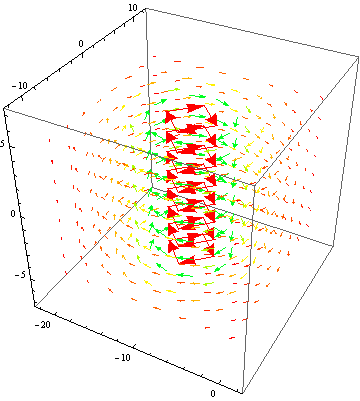
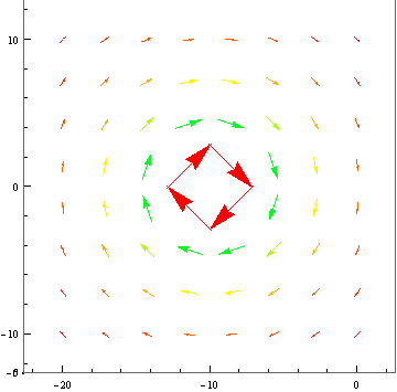
Where L is the instantaneous length of the loop along the rails, W is the rail separation (center to center), a is the radius of the rails, A is the cross sectional area of the rails, Qo is the initial charge in the capacitor, rho is the resistivity of the rails, v is the velocity, and C is the capacitance of the capacitor. We will then use this derived equation to solve for the force in two theoretical examples and provide simulations of the force as functions of time for each. For a small railgun, where a=.009, W=.03, C=450*10^-5 and Subscript[Q, 0]=1.8 we get
![\[ F=\frac{4 \left(\left(L \left(L^2-\sqrt{L^2+0.0009} L+0.0009\right)\right) \left(\frac{1.8 e^{-\frac{t}{(10 L+0.15) \rho }}}{(10 L+0.15) \rho }\right)^2\right)}{10^7 \left(\sqrt{L^2+0.0009} \left(\frac{9.04 k v}{10^{11} ((2 L+0.06) \rho )}+1\right)^2\right)} \]](https://pages.vassar.edu/magnes/wp-content/ql-cache/quicklatex.com-eea20afa2e0338d8725617d714207f8a_l3.png "Rendered by QuickLaTeX.com")
https://www.youtube.com/watch?v=LUhFbQCNXyg
However, although this is still more accurate than before, it is still not a completely accurate measure, as t and L are still expressed independently from one another. however, this issue may not be resolved as the equations of motion are too complicated to attain precise equations of motion.
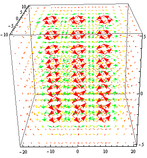
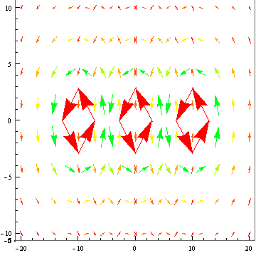
For the military railgun, however, the force is significantly greater, with a C=1.5 farads, Qo=10000, W=.8, and A=.01 additionally, the logarithmic terms were solved for to be inside of a range of values, which were then plotted as the variable k. Additionally, it should be noted that the values of the capacitance and charge are derived assuming a 100% conversion between energy stored in a capacitor and kinetic energy. The resistivity was plotted to be at a minimum that of Aluminum.
![\[ F=\frac{4 \left(\left(L \left(L^2-\sqrt{L^2+0.064} L+0.064\right)\right) \left(\frac{10000 e^{-\frac{t}{(75 L+60) \rho }}}{(75 L+60) \rho }\right)^2\right)}{10^7 \left(\sqrt{L^2+0.064} \left(\frac{4 k v}{10^9 ((2 L+1.6) \rho )}+1\right)^2\right)} \]](https://pages.vassar.edu/magnes/wp-content/ql-cache/quicklatex.com-4dfcfa30ba81fb63d151a85c3c3586e4_l3.png "Rendered by QuickLaTeX.com")
https://www.youtube.com/watch?v=0L6IaAcc59g
These measures of force are significantly more accurate than the theoretical version shown earlier in the data. The reason for this is that aside from the previous issue of L and t still being unrelated, this graph demonstrates the correct behavior for this system. We can manipulate the values of L however, and can see a clear trend in the force as a function of time in the above manipulation. Upon firing, the force quickly reaches a maximum as both the loop becomes large enough and the current still is present in sufficient quantity to provide efficient acceleration, however, as time goes and the loop size becomes larger, this term then collapses to be insignificant. That being said, it is clear that even a small system can accelerate objects to incredible velocity. Additionally, the resistance in the circuit must be accounted for as it has a tremendous impact on the graph of the force.
By combining and altering our manipulations of the equations given above, a clear trend in the force appears. Most likely, the force will resemble an overdamped wave, as seen in classical oscillations and EM waves. This means the force will reach a maximum, then exponentially decrease until the slug leaves the rails.
Finally, by analyzing these examples and the general equations of force it is clear that there is an ideal set of dimensions for a given system to maximize the force upon the slug. If each value falls outside the ideal range, the force will quickly decline by several magnitudes from the maximum possible force.
The Inductance Gradient
Remember the force can also be given as
![\[ F=\frac{1}{2} i L_1 t^2 \]](https://pages.vassar.edu/magnes/wp-content/ql-cache/quicklatex.com-f0022e1fd3dfa475bb6282811e1103ca_l3.png "Rendered by QuickLaTeX.com")
The other way to measure the force experienced by the slug in a railgun is using the inductance gradient, L’, for the railgun, by which you can find the optimal measures for a given system. The inductance gradient is measured in microhenries per meter, accounting for the Mu term of the force. For most cases, this value is calculated experimentally, however, for a miniscale railgun, the method of Lagrangian optimization. The object of this method is to minimize the value of the goal function,
![\[ \pmb{P=G+\sum _{i=1}^m \lambda _i\left(J_{\max }(h,w,z)_i-J_{\text{material}}\right)}\ \]](https://pages.vassar.edu/magnes/wp-content/ql-cache/quicklatex.com-403109457aa7117d5f953256a0fccbe4_l3.png "Rendered by QuickLaTeX.com")
The minimum of G is also proven to be the point of inflection in the P function. found using the second, series term of the P function. Eventually, this will form a regression, which can be evaluated using a system of equations to find the most efficient rail dimensions for a given system.
Where Jmax] is the maximum tolerable current density in the rails, and Lambda is an aribitrary constant. The Jmateral value is derived from the maximum tolerable current density of a copper cable (it comes from the material used in the system). The h, z and w, values are the dimensions of the rails. Jmax] is different from Jmaterial] because the current, attempting to take the shortest path through the system, will cluster in the corners between the rails and the slug.
Energy in a railgun
The most effective means to approximate the energy in the railgun is to use the capacitance and charge in the capacitor bank. Although this is extremely inaccurate while measuring the actual velocity and energy of the slug following firing of the system, it is an effective means to calculate the various constants going into the force. The muzzle energy can be calculated by measuring the kinetic energy of the slug following its expulsion from the loop, from this, it is possible to calculate the fraction of energy lost thermodynamically and frictionally in the system as discussed in the preliminary data. The energy in a capacitor is defined as:
![\[ W=\frac{Q^2}{2 C}=\frac{\text{CV}^2}{2} \]](https://pages.vassar.edu/magnes/wp-content/ql-cache/quicklatex.com-db8cfc58f990bf68ef6747fcd93f3131_l3.png "Rendered by QuickLaTeX.com")
The kinetic energy of any object is defined classically as:
![\[ T=\frac{\text{mv}^2}{2} \]](https://pages.vassar.edu/magnes/wp-content/ql-cache/quicklatex.com-a87d1fbd2829ef00c9f9b1e86085825d_l3.png "Rendered by QuickLaTeX.com")
Using this we can theoretically calculate the efficiency of both our large and small railgun systems. For the small system, where 10 400V, 450 microfarad capacitors are wired in parallel, C=4500 microfarads, V=4000 V, the mass is 3.6 grams and the muzzle velocity was around 700 m/s. This gives the following values:
![\[ W=\frac{\left(4\ 10^3\right)^2 4500}{10^6 2}=3.6 \text{kJ} \]](https://pages.vassar.edu/magnes/wp-content/ql-cache/quicklatex.com-0d3043e35968edb213e6a3be4d97b0f6_l3.png "Rendered by QuickLaTeX.com")
![\[ T=\frac{0.0036 700^2}{2}=882 J \]](https://pages.vassar.edu/magnes/wp-content/ql-cache/quicklatex.com-8b3b9ae4aef5ee95b05e7f934085fc42_l3.png "Rendered by QuickLaTeX.com")
![\[ \frac{T}{W}=0.245 \]](https://pages.vassar.edu/magnes/wp-content/ql-cache/quicklatex.com-d29ac6344d16a307a4a2b05d34bbbce5_l3.png "Rendered by QuickLaTeX.com")
For the small scale design, the system achieved a 25% efficiency in the transfer of energy. Although this appears to be a low efficiency, a standard firearm usually has an efficiency between 20-40%, and this is an extremely inefficient design for a railgun. The military, in their system tested in 2013, for which we modeled the forces earlier, the kinetic energy was given to be 33MJ however, due to the fact that the precise specifications of the capacitors are classified, we cannot effectively measure the efficiency of the system. Their efficiency is most likely higher, probably around 60%. The reason for this is that for high efficiency designs, the slug design and rail geometry changes significantly. We have modeled the military design as a square barreled launch system, with rails on either horizontal side. However, it is likely that the real geometry is different, to increase the efficiency of the discharge, as well as reduce the inevitable wear caused by heat. Additionally, rather than routing the current through the slug, through a gap all the while dealing with high resistances and thermodynamic loss, the millitary system insulates the main body of the slug, while adding a material at the rear which when subjected to the initial current shock will become a plasma. This is a much more efficient design, and that, along with the ability to make the slug more aerodynamically efficient will increase the total efficiency of the system. Although we do not have the tools to fully explain the resistivity of the plasma (plasma physics is a graduate level study), the Spitzer resitivity of a plasma is given as:
![\[ \eta =\frac{\Lambda \sqrt{m} \text{$\pi $Ze}^2 \ln }{\left(4 \pi \epsilon _0\right){}^2 \sqrt[3]{T k_b}} \]](https://pages.vassar.edu/magnes/wp-content/ql-cache/quicklatex.com-2a650db7f618ecba09d7471bda5aa7f1_l3.png "Rendered by QuickLaTeX.com")
*from http://silas.psfc.mit.edu/introplasma/ and Wikipedia, common knowledge to people who have taken plasma physics
Where Eta is the Spitzer resistivity, Z is ionization of nuclei, m is the electron mass, Curly Epsilon is the resistivity of free space, ln (Capital Lambda) is the Coulomb logarithm, k is Boltzmann’s constant and T is the temperature in kelvins. This value is presumed to significantly increase the efficiency. Additionally, the use of a plasma allows the system to be launched from rest, which as shown in the force approximations, significantly increases the efficiency of the system.
Acceleration on the slug
Using the derived equations of force found earlier, it is fairly simple to calculate the accelerations as functions of time in a railgun. Prior to showing, it ought to be noted that although the accelerations for even a small scale model are enormous, predicting in the hundreds of thousands, even tens of millions of metres per second squared, the slug only remains in the rails for periods best measured by microseconds, and the force dissipates even faster.
Given this understanding, the general form of the acceleration can be written as:
![\[ \text{Amag}=\frac{\mu _0 \left(L \left(-L \sqrt{L^2+W^2}+L^2+W^2\right)\right) \left(\frac{A Q_0 e^{-\frac{A t}{C \rho (2 L+2 W)}}}{\text{C$\rho $} (2 L+2 W)}\right){}^2}{m \left(\pi \sqrt{L^2+W^2} \left(\frac{A \mu _0 v \left((-\ln ) \left(L \sqrt{a^2+L^2}+L^2\right)+L \ln \left(\sqrt{(W-a)^2+L^2}+L\right)-\ln \left(L \sqrt{(W-a)^2+L^2}+L^2\right)+\ln \left(L \sqrt{a+L^2}+L^2\right)\right)}{4 \pi \rho (2 L+2 W)}+1\right){}^2\right)} \]](https://pages.vassar.edu/magnes/wp-content/ql-cache/quicklatex.com-8a0c4cd3269476be8ca2ae6a43730777_l3.png "Rendered by QuickLaTeX.com")
For our two examples, the smaller scale measure using a projectile weighing 3.6 grams and our large scale millitary model used a projectile mass of 3.2 kg. Subbing those in and generating manipulations, we arrive at:
![\[ \pmb{a=4*10^{-7}\frac{\left(L \left(.0009+L^2-L\sqrt{.0009+L^2}\right)\right)\left(\left(\frac{1.8}{(10L+.15)\rho }\right)e^{\frac{-t}{\rho (10L+.15)}}\right)^2}{.0036\sqrt{.0009+L^2}\left(1+\frac{1}{\rho (.06+2 L)}9.04*10^{-11} v k\right)^2}}\ \]](https://pages.vassar.edu/magnes/wp-content/ql-cache/quicklatex.com-2be65719b9a59c6cf68b0a279971c767_l3.png "Rendered by QuickLaTeX.com")
https://www.youtube.com/watch?v=18Ob75Vd8mE
for the small scale model, and:
![\[ \pmb{a=4*10^{-7}\frac{\left(L \left(.064+L^2-L\sqrt{.064+L^2}\right)\right)\left(\left(\frac{10000}{\rho (75L+60)}\right)e^{\frac{-t}{\rho (75L+60)}}\right)^2}{3.6\left(1+\frac{1}{\rho (1.6+2 L)}4*10^{-9} v k\right)^2\sqrt{.064+L^2}}}\ \]](https://pages.vassar.edu/magnes/wp-content/ql-cache/quicklatex.com-9f70801de53bb45c3dbc9b180570bb62_l3.png "Rendered by QuickLaTeX.com")
https://www.youtube.com/watch?v=uuEOy2nuuh8
For the military model. A is also the second time derivative of L as a function of T. So to find L(t), we can set up a differential using the acceleration to see if we can solve for theoretical values of velocity and position in the loop.
![\[ \partial L^2=\frac{\mu _0 \left(L \left(-L \sqrt{L^2+W^2}+L^2+W^2\right)\right) \left(\frac{A Q_0 e^{-\frac{A t}{C \rho (2 L+2 W)}}}{\text{C$\rho $} (2 L+2 W)}\right){}^2}{m \left(\pi \sqrt{L^2+W^2} \left(\frac{A \mu _0 v \left((-\ln ) \left(L \sqrt{a^2+L^2}+L^2\right)+L \ln \left(\sqrt{(W-a)^2+L^2}+L\right)-\ln \left(L \sqrt{(W-a)^2+L^2}+L^2\right)+\ln \left(L \sqrt{a+L^2}+L^2\right)\right)}{4 \pi \rho (2 L+2 W)}+1\right){}^2\right)}\partial t^2 \]](https://pages.vassar.edu/magnes/wp-content/ql-cache/quicklatex.com-0210475bca3ce06f034cdf640e540beb_l3.png "Rendered by QuickLaTeX.com")
where Mu, m, W, A, Rho, a, A, C, and Qo are constant with regards to t, while L and t are time dependent. This information, however does not help us solve this differential, which is impossible to be solved for. The real plots of position and time are almost always calculated experimentally, as are the inductance gradients. This is the most effective means to solve the system practically, as to arrive at our data, several simplifying assumptions had to be made.
Conclusions
The basic principles surrounding railgun physics are an excellent teaching tool to model much of the classical mechanisms of Electromagnetism. However, beyond the conceptual standpoint, the mathematics to calculate the specific quantities in the system are extremely complex. Since most of the variables are dependent upon one another, the resultant mathematics quickly expands into a long equations which cannot be computed. However, using the equations we have modeled, several understandings can be reached. First, the materials used in the railgun must be highly efficient conductors. Second, the geometry of the rails in question is crucial, helping determine the current densities, magnetic fields, forces and inductance gradient. Third, the force and resultant acceleration, when derived experimentally, should resemble an overdamped oscillator, where the system starts at 0, reaches a peak, then experiences an exponential decay. Finally, it is clear that for any railgun, regardless of setup, it can be assumed that there will be an enormous discharge of energy in an extremely small timescale, with forces anywhere from the hundreds of thousands to millions of newtons in the first few nanoseconds/ microseconds, depending on the size of the system. This last conclusion actually is the basis of the sub-field of engineering called pulsed power, which has a variety of applications.
Railguns, and by extension pulsed power, have a wide variety of uses. There is the obvious military benefit, being able to shoot kilogram sized objects with enough kinetic energy to annihilate most naval vessels at ranges previously limited to missiles. However, this technology is not only useful for that application. In a more optimistic setting, these systems can be used to quickly and cheaply accelerate objects into space (non-living, as the forces experienced to accelerate organic matter to escape velocity would most likely result in immediate death), Finally, and perhaps most interestingly, railguns have been proposed as starter mechanisms for fusion reactors, specifically inertial confinement systems. Using a railgun, the idea is to collide plasmas at high velocity into a single locus, hopefully triggering a self sustaining fusion reaction. Fusion is, of course the holy grail of energy research, and the invention of a self sustaining reactor would be a significant leap in technological progress.
Finally, although we had planned to regroup and construct a railgun, we simply ran out of time as well as material issues. We sent a request for materials into the associated offices on campus, and they responded on May 2nd. As such, we were under enormous stress to undertake that portion of the project. Although we gathered most of the necessary materials, there were several issues with assembly. First, we had to use a flash circuit as the basis for our railgun, unfortunately, in order to expose all the necessary terminals, the circuit had to be exposed. Additionally, the specific camera we used always had charge within the capacitor. As such, I shocked myself, a lot. Following this issue, we discovered that although the base components were available on campus, wiring that was appropriate for the circuit was being used both in the electronics lab, and the physics department. We then had to cut most of the circuit. Finally, we managed to make a semi-functional railgun; however, the slug possessed too high of a resistivity, and was too massive. So there was no launch, this limited our project’s scope, as most of the values for the railgun’s dimensions must be determined experimentally, as there are simply too many variables to cope with.
However, it is still possible to understand most of the railgun system using theoretical derivations. It became clear that when trying to design a system to deliver huge quantities of energy in a short time railguns are the ideal system, assuming there has been careful consideration given to the systems dimensions.
Mathematica notebook:
https://drive.google.com/a/vassar.edu/#folders/0B0K4JjJfDy1fNnE4MHJON0k4TDg


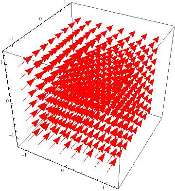
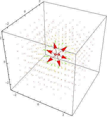


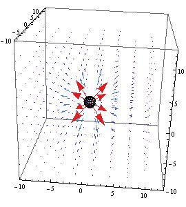
![\[ \textbf{E} = \frac{q_e}{\epsilon_0 4 \pi r^2} \textbf{$\hat{r}$} \]](https://pages.vassar.edu/magnes/wp-content/ql-cache/quicklatex.com-3e809ffe305a5dd257991f875380bb3e_l3.png "Rendered by QuickLaTeX.com")
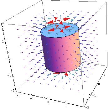
![\[ \textbf{E} = \frac{\rho R^2 }{2r\epsilon_0} \textbf{$\hat{r}$} \]](https://pages.vassar.edu/magnes/wp-content/ql-cache/quicklatex.com-555b4e970293d3e4e78338dd68259d29_l3.png "Rendered by QuickLaTeX.com")
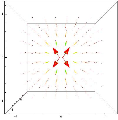
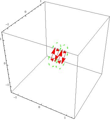
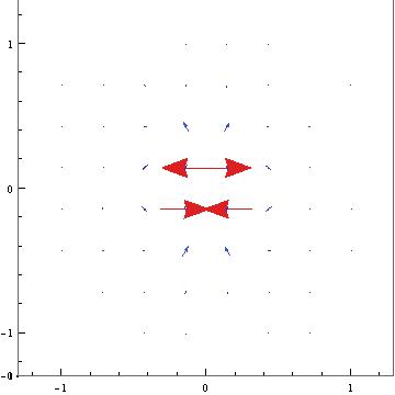
![\[ V = \frac{p_o \cos(\theta)}{\epsilon_0 4 \pi r^2} \]](https://pages.vassar.edu/magnes/wp-content/ql-cache/quicklatex.com-e0d3b83684360e0a3e0cfeac94fc47a1_l3.png "Rendered by QuickLaTeX.com")
![\[ V = \frac{p \cos(\theta)}{r^2} \]](https://pages.vassar.edu/magnes/wp-content/ql-cache/quicklatex.com-17a8904c297439b92bb61b4fbb16897e_l3.png "Rendered by QuickLaTeX.com")
![\[ \textbf{E} = -\nabla V \]](https://pages.vassar.edu/magnes/wp-content/ql-cache/quicklatex.com-4af224d44a6a6606401ab97bc7cbea18_l3.png "Rendered by QuickLaTeX.com")

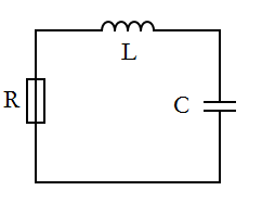
 [1]
[1]![\text{DSolve}\left[\frac{\text{Current}(t)}{\text{Capacitance}}+\text{Inductance} \text{Current}''(t)+\text{Resistance} \text{Current}'(t)=0,\text{Current}(t),t\right]](https://pages.vassar.edu/magnes/wp-content/ql-cache/quicklatex.com-edf43b2ac32669349aa6c8d04ba9e32e_l3.png "Rendered by QuickLaTeX.com") [2]
[2] [3]
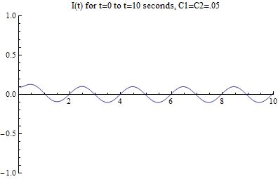
[3] . So, the initial current in the circuit must be 0.1 amps. Using a graphical guess-and-check method in Mathematica, I determined the value of the two constants to be approximately 0.05 each, resulting in a solution that is given by
 [4]
[4]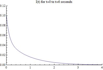
 [5]
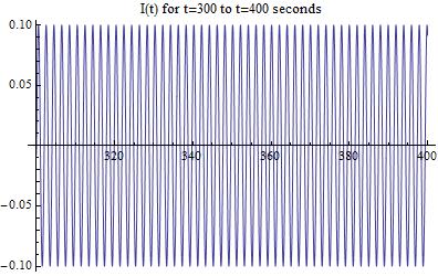
[5] is the resonant angular frequency,
  is an initial value dependent on the voltage source, and t is the time. The inductance (L), resistance (R), and capacitance (C)are all determined by their respective circuit components, which are easily changed out for different ones.
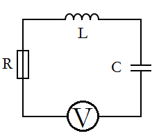
  [6]
[6] ).
).![\text{DSolve}\left[\frac{\text{Current}(t)}{\text{Capacitance}}+\text{Inductance} \text{Current}''(t)+\text{Resistance} \text{Current}'(t)=E_{0} \omega \cos (\omega t),\text{Current}(t),t\right]](https://pages.vassar.edu/magnes/wp-content/ql-cache/quicklatex.com-4fd6cd2ab6f0ba47fdfaab15b71e9d9e_l3.png "Rendered by QuickLaTeX.com") [7]
[7] [8]
[8] [9]
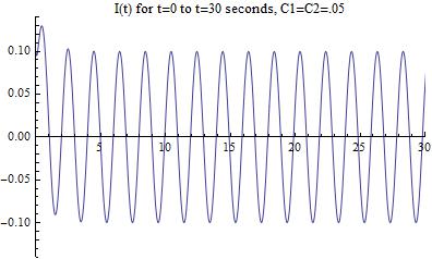
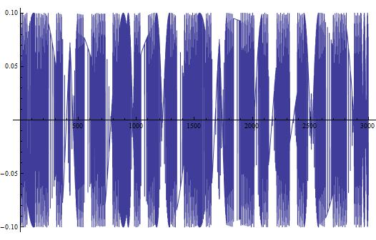
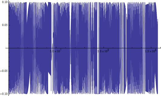
[9] . However, we can approximate the equation by only looking at the last term, which is a superposition of sin and cosine functions along with a couple exponential terms thrown in. The reason that we can apply this approximation is that the first two terms “damp out” quickly, and thus have exponentially less of an effect as time progresses. The reader may still be curious to see how much of an effect these terms have on the current flowing through the system: to that I say don’t worry! After my initial approximation, I will solve for these constants and compare the two cases.
 [10]
[10]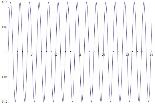
![C[1]](https://pages.vassar.edu/magnes/wp-content/ql-cache/quicklatex.com-86d57aecc373976151de585b5b2bec5a_l3.png "Rendered by QuickLaTeX.com") and
and ![C[2]](https://pages.vassar.edu/magnes/wp-content/ql-cache/quicklatex.com-12b2dbf736e307ece734ae42b09665aa_l3.png "Rendered by QuickLaTeX.com") and figure out graphically what they should be.
and figure out graphically what they should be. [12]
[12]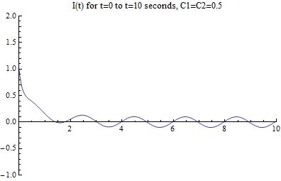
 [13]
[13]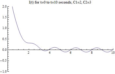
 [14]
[14]