Category Archives: Project Plan

Ultrasonic Analysis

Introduction

The Fourier Transform (FT) is a mathematical tool that takes a signal in a time domain and decomposes it into it’s frequency domain. Below is the definition of the continuous FT of $x(t)$ to $X(f)$,

$X(f) = \int_{-\infty}^{\infty} x(t)e^{-i2\pi ft}~dt$.

This comes in handy when trying to analyze signals found found in electrical circuits, diffraction patterns, and sound waves. We intend to use the same techniques to study and manipulate sound signals found in the ultrasound domain.

Acoustics is the study of the generation, transmission, and reception of vibrational waves in a medium. Mostly acoustics is associated with sounds we can hear, but vibrational waves can occur outside of the range of human hearing. Humans detect vibrational waves from a range of 20Hz to 20,000Hz as sound waves, but any vibrations occurring above or below this frequency band go undetected by our ears. Ultrasound is any sound vibration above 20,000 Hz, it shares all physical properties of audible waves other than human perception.

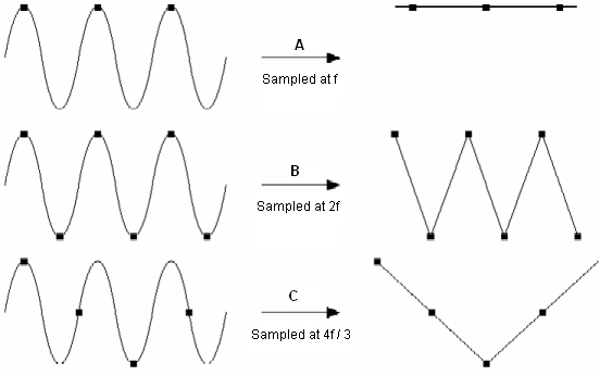
The standard sampling rate used by computers to capture sounds vibrations is 44.1 samples per second. It is necessary to capture signals slightly above the nyquist frequency. The nyquist limit is a result of having to sample a wave at least twice per cycle to represent the wave without aliasing. The nyquist limit will be an important part of accurately recording the waves because of the high frequency content of ultrasound.

Here is a small demonstration the shows the importance choosing a sampling frequency

Determining the sampling rate of these signals will be an important experimental consideration, but we know it will be much greater than 44.1 samples per second.

Goal

We will be processing a variety ultrasound frequencies and attempt to pitch shift them down (without loss of quality) to the audible range for listening.

Timeline

Week 1 (4/6 – 4/12)

Gather necessary resources and work on problems from the texts to gain requisite background information and foundational code to perform effective analysis of ultrasound signals.

Week 2 (4/13 – 4/19)

Continue to work on the code. Study sources that generate ultrasonic sound vibrations, and methods of recording them.

Week 3 (4/20 – 4/26)

Record ultrasound signals and convert recordings into a suitable file for matlab to take in for analysis. Attempt to analyze and pitch shift the signal and play it back. Debug errors.

Week 4 (4/27 – 5/3)

Continue analysis on a variety of signals recorded during week 2.

Week 5 (5/4 – 5/10)

Presentation and write-up.

Resources

Fundamentals of Acoustics 4th Edition by L. E. Kinsler and A. R. Frey

A Student’s Guide to Fourier Transforms 3rd Edition by J. F. James

Fundamentals of Digital Signal Processing Using MATLAB®, 2nd Edition by Schilling/Harris                  

Computational Physics 2nd Edition by Nicholas J. Girodano, Hisao Nakanishi

The Computer Music Tutorial by Curtis Rhodes

Share

Physics of Baroque Keyboard Instruments: Project Plan – Kachelein

Introduction

– In chapter 6 of the class text, we were first introduced to the motions of waves on strings, even modeling their motion in a few simple cases. In chapter 11, the physics of musical instruments is explored. The guitar and the piano are featured prominently in this chapter, as they have relatively simple mechanics and are stringed, hence the framework for exploring their behavior has been established. Other instruments, each with different physical characteristics, can also be modeled. The goal of my project is to start with information in chapter 11 and build full, working models of the harpsichord, clavichord and, hopefully, the pipe organ, three instruments with which I am very familiar. The final aim of the project is to compare computed data with actual signals from the instruments in question, verifying (or nullifying) the computational models.

Methods

– MATLAB will, of course, be used as the primary, if not sole, computational tool (if a difficult differential equation needs to be solved, Mathematica may be invoked). For the harpsichord, a model for the plucking force will need to be built (harpsichord strings are plucked, rather than struck like those of a piano). Though plucked strings are already discussed in the guitar sub-chapter, I feel that a more complicated but realistic model can be built (for example, by considering the effect of the plectra as the string slides off of it). The string’s motion will be governed, naturally, by the wave equation:

which is computationally realized by eq. 6.6:

– The clavichord is also a string instrument which has a striking mechanism like that of the piano, but which is physically much different. In particular, the forcing site is also a boundary of the string, so a radically different model from that of the piano/harpsichord may or may not need to be used.

– If the organ proves feasible after addressing the instruments above, I will attempt to model at least one type of pipe and at most two types (round metal and square wooden pipes). Part of chapter 11 addresses a one dimensional pipe, and the methods are claimed to be easily extendable to three dimensions using coupled partial differential equations. For the one dimensional case, we have pressure, p, and velocity, v, in air of density ρ and sound speed c given by:

which has a numerical form given by equation 11.37 in the book:

where Z is acoustic impedance, the correct value of which will be of particular importance (material dependent).

– The experimental portion of the project is not yet laid out. I may request assistance from Professor Bradley in taking and analyzing acoustic signals from the aforementioned instruments. Regardless, I intend to compare the Fourier transforms of actual signals to the computed transforms in order to see if the peak frequencies match.

Time Line

– Week 1: Practice by completing a few problems from chapter 11.

– Week 2: Build a working model for the harpsichord, as complete as the piano model in the book, and take data. Begin work on clavichord model.

– Week 3: Complete clavichord model. Begin organ model.

– Week 4: Complete organ model. Record real instruments to compare to models.

– Week 5: Compare experimental data to models. Allow time for write up and possible revision of models.

– Week 6: Further time, submit Wednesday.

Resources:

– Giordano N J, Nakanishi H. “Computational Physics, 2nd Edition.” 2005. Addison-Wesley. ISBN-10: 0131469908.

– MATLAB R2014b by MathWorks®

Share

Project Plan

Measuring and Modeling Physical RCL Circuits

Purpose and Goals:

The purpose of this project is to demonstrate the difference between theoretical descriptions/relationships of basic LC circuits and experimental values. This is also an exercise in developing a deeper understanding of the theoretical equations governing these relationships. I will record the voltage drop across various components in each circuit and plot them in comparison to the theoretically predicted values. In addition, I will try to answer questions such as “What are the probable causes for deviation from predicted values?”

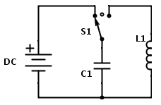
The first and most simple circuit I will work with is a basic LC circuit:

EM circuit DC

The DC power source charges the capacitor until it is discharged (via switch) into the right hand circuit. In theory the current should oscillate back and forth between the capacitor and inductor indefinitely if there was no resistance in the circuit. Actual experimental measurements should reveal some resistance due to the wires and components themselves. Below is the start of my derivations for the voltage across each components:

Kirchoff’s Loop Law states that the total voltage drop across the right hand circuit loop should be zero:

\Delta V_{L}+\Delta V_{C}=0       (1)

We know that the voltage drop across an inductor is equal to L(dI/dt) and across a capacitor is Q/C:

 L\dfrac {d^{2}Q\left( t\right) } {dt^{2}}+\dfrac {Q\left( t\right) } {c}=0     (2)

Which can be rewritten as

\dfrac {d^{2}Q\left( t\right) } {dt^{2}}+\omega _{0}^{2}Q\left( t\right) =0     (3)

Leaving us with the general solution to this second order differential equation

Q\left( t\right) =Q_{0}\cos \left( \omega _{0}t-\delta \right)      (4)

The derivation of the above equations will be more thorough in future posts.

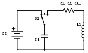
RLC circuit

This circuit is dampened with a resistor, and thus no longer resembles simple harmonic motion, but rather a damped harmonic oscillator.

EM circuit DC R


Kirchoff’s Loop Law now reads

\Delta V_{L}+\Delta V_{R}+\Delta V_{C}=0     (5)

 L\dfrac {dI} {dt}+RI +\dfrac {Q} {C} =0     (6)

Which leaves us with a new second order differential equation

 L\dfrac {d^{2}Q\left( t\right) } {dt^{2}}+R\dfrac {dQ\left( t\right) } {dt}+\dfrac {Q\left( t\right) } {c}=0    (7)

\dfrac {d^{2}Q\left( t\right) } {dt^{2}}+\dfrac {R} {L}\dfrac {dQ\left( t\right) } {dt}+\dfrac {1} {LC}Q\left( t\right) =0    (8)

\dfrac {1} {LC}\equiv \omega _{0}^{2}   (9)

\dfrac {R} {L}\equiv 2\beta     (10)

\dfrac {d^{2}Q\left( t\right) } {dt^{2}}+2\beta \dfrac {dQ\left( t\right) } {dt}+\omega _{0}^{2}Q\left( t\right) =0    (11)

Eq. (11) is the second order differential equation governing the charge on the capacitor as a function of time and thus describing the voltage drop and current through the other components of the circuit.

Predictions

Theoretically I should expect the voltage across the components in an LC circuit to oscillate indefinitely according to simple harmonic motion. I expect that with a real circuit this would not be the case. A physical LC circuit would actually behave as if a resistor was in series with the two components, causing the amplitude of the oscillations to decrease over time. This is because the circuit parts, such as the wires connecting each component, are not ideal and have resistance.

I predict that a graph of the voltage difference over time for a given component will appear as a decaying sinusoidal wave. In other words it should resemble an dampled oscillation.

Methods

I will use a PicoScope digital oscilloscope to measure the voltage difference across the capacitor in the LC circuit. In this way I will both be able to see the voltage the capacitor is initially charged to as well as record the transition from a steady voltage to an oscillating voltage.

Sources, Resources, and Parts Needed

Equipment Needed:

  • DC power source, AC frequency generator, Oscilloscope, Computer, Multimeter

Parts Needed:

  • Breadboard; various values of resistors, capacitors, and inductors; switch; wires/alligator clips

Helpful Texts:

  • Physics for Scientists and Engineers: A Strategic Approach with Modern Physics (2nd ed.) by Randall D. Knight
  • Introduction to Electrodynamics (4th ed.) by  David Griffiths
  • Data Reduction and Error Analysis for the Physical Sciences by Philip R. Bevington, D. Keith Robinson
  • Experimentation : an introduction to measurement theory and experiment design by D.C. Baird
  • Ordinary Differential Equations by Morris Tenenbaum and Harry Pollard
  • Class notes – Classical Mechanics (PHYS 210), Zosia Krusberg.

Websites:

Timeline

Week 1 – April 20th-26th. Acquire all equipment and parts needed for experiment: Talk to Larry Doe for parts and possibly a power source. Talk to David Rishell about an AC signal generator. Setup experiment in Mudd 216 with Prof. Magnes’ oscilloscope, DC power source, and multimeter.

Week 2 – April 27th-May 3rd. Derive equations to predict voltage drop across components to plot on top of collected data. Those equations being ΔV for LC, dampened LC (RLC), and AC driven RLC in series circuit. Collect data on voltage drops across LC and dampened LC circuit components. Plot data in mathematica.

Week 3 – May 4th-10th. Collect data on voltage drops over AC driven circuit. Predict resonance frequency. Define equations governing resonance frequency and find actual resonance frequency of circuit. Plot findings in mathematica. Consider sources of error or causes of deviation from predicted values on all three circuit configurations.

Week 4 – May 11th-17th. Finish data collection and additional exploration/inquiry. Create time dependent plots in mathematica to demonstrate projected vs experimental values.

Place/Logistics

Experimentation and data collection will occur in Professor Magnes’ lab in Mudd 216. Brian and Tewa generally work MWF and can be contacted for access to the lab.


Share

Revised Project Plan: Relativistic E&M

So it seems that step 1 of my original plan is more involved than I thought. To satisfactorily derive the E- and B-field transformation equations, it would be necessary to delve into the depths of relativistic mechanics, including the transformation of equations for motion, momentum, and energy, among others. This seems like it is outside the scope of the project: indeed, Griffiths spends about 55 pages before he is able to state the field transformation equations. I thought there would be a point halfway through at which I could pick up and start the derivation, but I was incorrect, so I am going to take the transformation equations as given, and work from there.

That being said, my new timeline will be essentially the same as the old one, just starting at what used to be Step 2 with the application of the transformation equations to one or two situations.

1) 4/14-4/18: Pick one or two simple scenarios and find their E- and B- fields if they were traveling in a moving reference frame. This will be a computational step. The transformation equations are pretty straightforward, so it should take less time. This is just to have a proof of concept, so it is less important that the system has interesting behavior in a moving reference frame.

2) 4/18-4/24: Make 3D or 2D vector field models of these situations in Mathematica. This portion will be focused on figuring out how to make mathematica do what I want. The goal is to come up with an animation or interactive figure that can be used to view the vector fields when the system is moving at different speeds, starting at non-relativistic speeds and working up to the speed of light.

3) 4/24-5/2: Find and model situations that display either representative or unusual behavior when considered in a relativistic reference frame. Once the Mathematica simulation for the first situation has been figured out, the following cases should be easier to take care of. Interesting behavior might include systems that only have an electric field in one reference frame and only a magnetic frame in another. It also may be interesting to consider what happens if a reference frame is moving faster than the speed of light.

4) 5/15/14: Summarize results and write conclusions. This will consist of a final look at the systems considered earlier and suggest possible directions for future exploration.

Share

Project Plan: Van Allen Belts

Summary:

The primary goal of my project is to create a 3d model of the shape and strength of the Earth’s magnetic field and define the locations of the Van Allen Belts within that model. According to the research I have done so far, a planetary magnetic field resembles the field of cylinder. Applying relevant Earth properties, I would then be able to create an initial model of the field.  Furthermore, due to the proximity of these belts to the Earth, I will not have to take interactions with the solar wind into account when modeling the field. The modeling will be done with the Mathematica program. With the model complete, I would hope to compare it to other, more exact models of the Earth’s magnetic field to confirm the theoretical location of the Van Allen Belts. I would also be interested in noting if there is any relationship between core size of the planet and development of a magnetic field. My current research hasn’t turned up any leads for a mathematical way to approach this problem however.

Timeline:

•Week  1: (week of 4/6) Research the Van Allen Belts and Define Project Parameters -During this first week I plan to research the different possible facets of my project in order to determine the particular parameters I will be creating the 3d model with. This also includes looking for previously made 3d vector fields that can teach me how to plot the vector field in Mathematica. Furthermore I will be looking into some of the secondary objectives of my project to see if the ideas can be executed in a reasonable amount of time.

•Week 2: (week of 4/13) Creating the Initial 3D Model – During the second week of the project, we proceed onto the next step of creating our basic 3D magnetic field model. This 3D vector field model will be created using Mathematica and will create a visual representation of the Earth’s magnetic field. The initial model will be based off of the magnetic field of a cylinder, a design which has been suggested by multiple sources.

•Week 3: (week of 4/20) Finishing the Initial 3D Model and Model Comparisons – This week will be used to put any necessary finishing touches on the initial model and determine the location of the Van Allen belts within the model. I will also be comparing the model to observed data and other proposed models of the field. From these findings, I will be able to determine the accuracy of the field modeled in Mathematica. If the simple cylindrical model is not as accurate as predicted, this week will also be taken to edit the model and improve its accuracy.

•Week 4: (week of 4/27) Extended Modeling – During this week I will finish all alterations on a final edited model. If there is extra time, the current plan is to systematically alter the model to see how certain changes effect the magnetic field. Specifically my goal is to see if there exists some sort of correlation between the planet’s core size and the development of its magnetic field and subsequently its Van Allen Belts. If a correlation like this can be seen, the magnetic fields of other planets will be modeled and compared to actual data. This will allow us to confirm if the created model can be applied to other planets with only minor alterations to its coding.

•Week 5: (week of 5/4) Finishing Touches – During this week, any extra modeling will be quickly finished up and the rest of the week will be dedicated to organizing the collected data into a final presentation.

Sources:

Currently the sources I have browsed are:

http://www.phy6.org/Education/Iradbelt.html

http://vanallenprobes.jhuapl.edu/science/overview.php

https://www.spenvis.oma.be/help/background/traprad/traprad.html#APAE

http://www.nasa.gov/mission_pages/rbsp/main/index.html#.U0O-7fmIDlx

Share

Project Plan: A Guide To Convolution In Action

Description of project

Convolution is the theory behind interpreting the data presented. When physicists use optical tools for their experiments they need to understand whether the optics they are using will transmit the proper information. In practice one is limited to the material of the filters, as the wave fronts get distorted by the material they pass through. In order to be able to work with what you have, physicists model their possible optics layout before purchasing the optics. To retrieve the desired information physicists model the convoluted wave front, and then prepare a good deconvolution mechanism that in practice should yield the necessary data. This project is an attempt to understand convolution and deconvolution of electromagnetic waves through optical filters. I will be exploring the theory behind convolution, demonstrate examples of convolution, attempt deconvolution of a convoluted distributions, and then hopefully show a real world example of actual optical filters.

Theory

Convolution is the mixture of functions that individually have known Fourier transforms. A Fourier transform is the transformation of a square-integrable function f(x) from one domain to another (5). It is defined as such:

f(x)=\frac{1}{\sqrt{2\pi}}\int_{-\infty }^{\infty }\!\Phi(k)e^{ikx}dk \qquad \Phi(k)=\frac{1}{\sqrt{2\pi}}\int_{-\infty }^{\infty }\!f(x)e^{-ikx}dx

Both the function and the Fourier transform describe the same system though under different but related spaces (See: Plancherel’s Theorem). The advantage is if you have a machine that measures time but you are trying the measure the system as a function of frequency, then you can measure the system with that machine and simply take the Fourier transform of your data. Unfortunately, the deviations of the Fourier pairs are bounded by the uncertainty principle. A function with a narrow spread will yield a transformation with a wider spread, and vice versa.

\sigma^2_\Psi\sigma^2_\Omega\geq\left(\frac{1}{2i}\langle[\hat{\Psi},\hat{\Omega}]\rangle\right)^2

where \hat{\Psi} and \hat{\Omega} are two arbitrary operators, and \sigma_{i} is the standard deviation.

The definition of a convolution of two functions is defined as follows:

f_{1}(x)\ast f_{2}(x)=\int_{-\infty }^{\infty }\!f_{1}(x')f_{2}(x-x')\mathrm{d}x' \\ \\ \Phi_{1}(k)\ast \Phi_{2}(k)=\int_{-\infty }^{\infty }\!\Phi_{1}(k')\Phi_{2}(k-k')\mathrm{d}k'

The convolution theorem then states that the Fourier transform of a convolution is the product of the Fourier transforms to a factor of \sqrt{2\pi}. Similarly, the Fourier transform of a product of functions is the convolution of the Fourier transforms (5):

{\widehat_{f_{1}\ast f_{2}}} (x)= \sqrt{2\pi}\;{\Phi_1}(k)\cdot {\Phi_2}(k)  \qquad {\widehat_{f_{1}\cdot f_{2}}} (x)= \frac{1}{\sqrt{2\pi}}\;{\Phi_1}(k)\ast {\Phi_2}(k)

The implication of this theorem is if any arbitrary curve can be expressed as a product of functions with given Fourier counterparts, then it can undergo deconvolution to yield the desired data as represented by known functions (3).

f_{1}(x)\ast f_{2}(x)\rightleftharpoons \Phi_{1}(k)\cdot \Phi_{2}(k)

Timeline

 All work will either be done on my computer or at the sci-vis lab.

Week 1: I will become familiar with Professor Magnes’s MATLAB script and reconstruct it in Mathematica. I will use the information provided for me in the texts to create new examples of various convoluted distributions. I will also provide an introduction to the theory that pertains to my project.

Week 2: By now I should be familiar enough with Mathematica to display some cool examples. I will attempt to provide an example of real world convolution of two optical filters from thorlabs. In practice convolution of two actual filters is not as easy as adding two equations. I will need to figure out how to generally apply my ideal examples to sets of data.

Week 3: I will now attempt to demonstrate the deconvolution of a distribution. I will show this by using one of my previous examples. In theory I should be able to demonstrate proper deconvolution of two functions.

Week 4: Now that I have demonstrated deconvolution, I should be able to demonstrate deconvolution of the data I had previously showed in convolution form. This would be very tricky but hopefully I should be able to succeed.

Week 5: I may be setting the bar up too high, so possibly some of my work will take more time than expected. I should be finished with everything now. Here I will tweak my project, and conclude my demonstration.

Note: I may stray from my timeline, but that is only because I got caught up in an interesting phenomenon. Should I decide to alter my direction, I will update my timeline accordingly.

Resources

Will be updated if necessary

(1) Griffiths, David J. Introduction to Electrodynamics. Upper Saddle River, NJ: Prentics Hall, 1999. Print.

(2) Hecht, Eugene. Optik. München: Oldenbourg, 2001. Print.

(3) James, J. F. A Student’s Guide to Fourier Transforms: With Applications in Physics and Engineering. Cambridge: Cambridge UP, 2011. Print.

(4) Pedrotti, Frank L., Leno S. Pedrotti, and Leno Matthew. Pedrotti. Introduction to Optics. Upper Saddle River, NJ: Pearson Prentice Hall, 2007. Print.

(5) Sadun, Lorenzo Adlai. Applied Linear Algebra: The Decoupling Principle. Providence, RI: American Mathematical Society, 2008. Print.

Question to the reader: Is the verb of deconvolution: deconvolve or deconvolute?

Share

Project Plan: RLC Circuits

Plan/Goals:

In this project, I plan to study the relevant differential equations that govern RLC circuits and use Mathematica to solve them for values that are useful. The general equation governing a basic RLC circuit with a capacitor, voltage, resistor, and inductor in series, in that order is:

LI'(t)+RI(t)+\frac{1}{C}Q(t)=V(t) [Equation 1] (UBC- Source 4)

which, when going through a series of substitutions, becomes:

LI''(t)+RI'(t)+\frac{1}{C}I(t)=\omega E_{0}cos(\omega t) [Equation 2] (UBC- Source 4)

Equation 1 has six variables: L (inductance), R (resistance), C (capacitance), V (voltage), Q (charge), and I (current). When a circuit like this is set up in the lab, the values that are known are L, R, C, and V because they directly depend on the components of the circuit. Once the differential equation [2] is solved, values for current (I) and charge (Q) can be determined. I will use Mathematica to solve for the general solution to this differential equation [2], which is a second-order differential equation. Once I have the general solution, I will vary the initial conditions to determine the effect of different circuit components on the overall properties of the circuit. Following this, I will develop more series RLC circuits with components that are set up differently in terms of their component structure.

Timeline (Weeks 1-5):

Week 1: I will begin by reviewing basic differential equation solving techniques for first and second order differential equations. I will also study the differential equation solving capabilities of Mathematica and review the techniques for solving second-order differential equations as they apply to RLC circuits.

Week 2: I plan on solving for the general solution to Equation 2 above (using Mathematica). I will vary different initial conditions and create graphs that visualize the changes that occur. I will also have a visual representation of the circuit.

Week 3: Develop another series circuit or study a previously built one. Determine the general equation for it and begin the solution process.

Week 4: Finalize the solution for the second circuit. Develop graphs for visualization purposes.

Week 5: I will finalize my project by proofreading all the components and making sure everything is presentable. I will also provide constructive criticism to my peers on their projects.

Sources:

1. Mathematica Cookbook by Sal Mangano

2. Electronic Circuit Analysis for Scientists by James A. McCray and Thomas A. Cahill

3. Dynamical Systems with Applications using Mathematica by Stephen Lynch

4. The RLC Circuit- University of British Columbia- http://www.math.ubc.ca/~feldman/m121/RLC.pdf

5. Class Notes- Mathematics 228 (Methods of Applied Mathematics) taught by Matthew Miller

Collaborators:

N/A


Share

Project Plan: Relativistic E&M

Sources: In terms of sources, this project is fairly simple. The main source will be Chapter 12 of Griffiths’ Introduction to Electrodynamics, 3rd ed. This will provide a framework for deriving the transformation equations.

Process/Timeline: There are five main steps involved in this project:

1) 4/7-4/14: Derive the transformation equations. This will be a proof-based step, and I need to refresh myself on some of the concepts of mechanical relativity, so it may take some time.

2) 4/14-4/18: Pick one or two simple scenarios and find their E- and B- fields if they were traveling in a moving reference frame. This will be a computational step. The transformation equations are pretty straightforward, so it should take less time. This is just to have a proof of concept, so it is less important that the system has interesting behavior in a moving reference frame.

3) 4/18-4/24: Make 3D or 2D vector field models of these situations in Mathematica. This portion will be focused on figuring out how to make mathematica do what I want. The goal is to come up with an animation or interactive figure that can be used to view the vector fields when the system is moving at different speeds.

4) 4/24-5/2: Find and model situations that display either representative or unusual behavior when considered in a relativistic reference frame. Once the Mathematica simulation for the first situation has been figured out, the following cases should be easier to take care of. Interesting behavior might include systems that only have an electric field in one reference frame and only a magnetic frame in another. It also may be interesting to consider what happens if a reference frame is moving faster than the speed of light.

5) 5/15/14: Summarize results and write conclusions. This will consist of a final look at the systems considered earlier and suggest possible directions for future exploration.

Share

Project Plan: Electric & Magnetic Field Modeling

Sources:

  • Introduction to Electrodynamics by David J. Griffiths, Fourth Edition: Chapter 5

Model:

I will be creating models of the magnetic fields of a bar magnet, sphere and a cylinder. Each of these fields will be first be derived for continuous distributions and then modeled on Mathematica using its Vector Field plot function in 2 and 3 dimensions. Time-permitting, I will also model the magnetic fields for distributions that are not continuous (perhaps with varying current densities dependent on space J(r)). Example systems can be found in Griffiths’ Introduction to Electrodynamics exercises.

Timeline:

April 7-April 14: Complete project proposal and begin derivations

April 14-April 21: Alter project proposal as needed and complete derivations

April 21- April 28: Post derivations and begin Mathematica modeling

April 28-May 5: Final Mathematica modeling and combination with Peter’s Modeling

Collaborators:

I will be working with Peter Florio, who will derive and model the electric fields of the same distributions. We plan to compare our results side-by-side to observe the similarities and differences between our models and to notice the parallels in our derivations.

Share

Project Plan: Modeling Electromagnetic Fields for Spherical Objects

Sources

I will be utilizing Introduction to Electrodynamics, 4th Edition, by David J. Griffiths. Specifically, I will begin with Gauss’s Law, as defined by Griffiths on page 69:

$ \oint \! \textbf{E} \cdot \mathrm{d} \textbf{a} = \frac{1}{\epsilon_0} Q_{enc} $

Further, I will utilize the formula for the electric field of a point charge below (found on Griffiths page 72), which can be generalized for a spherical object:

$\textbf{E} = \frac{1}{4 \pi \epsilon_0} \frac{q}{r^2} \mathbf{\hat{r}} $

I will additionally work with the magnetic field for the spherical object. Griffiths (page 263) gives the average magnetic field due to uniform current over a sphere as:

$ \textbf{B}_{ave} = \frac{\mu_0}{4 \pi} \frac{\textbf{m}}{R^3}$

Where m is the total dipole moment of the sphere and R is the radius of the sphere.

I will be using Mathematica 9 as my modeling tool.

Plan of Action

I will begin by using the equations above to start with modeling the electric field of a point charge. From there, I will model the electric field for a hollow spherical object. I will create a manipulatable object in Mathematica for changes in radius and charge. I will then move on to modeling the average magnetic field for a spherical object, and attempt to create a manipulatable object akin to the one for electric fields. Next, I will model the electric and magnetic fields for concentric spherical objects, with the goal of ultimately coming up with a very liberal approximation for modeling the magnetic field of the Earth, if the Earth is thought of as several concentric spheres (due to the crust, mantle, and outer/inner cores). However, this will only occur if time permits, as will a preliminary examination of dielectrics.

Timeline

Week 1 (4/6-4/12): Work on the simplest case of a point charge, and learn to work within Mathematica

Week 2 (4/13-4/19): Work to create manipulatable object for electric field of sphere, and begin working on modeling the average magnetic field for a spherical object with uniform current density

Week 3 (4/20-4/26): Model electric and magnetic fields of concentric spherical objects, submit preliminary results on Tuesday on blog

Week 4 (4/27-5/3): Wrap up, submit final data and conclusion on Wednesday, dielectrics if time permits

Collaborators

I am working with Brian Deer, who is focusing on bar magnets, and Tewa Kpulun, who is focusing on cylindrical objects. We will be meeting weekly to discuss our progress, share Mathematica-related insights, and help each other in whatever ways we can.


Share