Background Information:
Earth’s Van Allen Belts are a naturally occurring phenomena due to the presence of the Earth’s magnetic fields. Specifically, they are two zones of space where large concentrations of high energy particles are trapped by the magnetic field lines of our planet. The zones are defined by our field lines; toroidal in shape, and encompass the planet at particular radii from the surface. Following the field lines, the regions begin from Earth’s Southern Pole and loop to its Northern Pole This is illustrated in the diagram below.
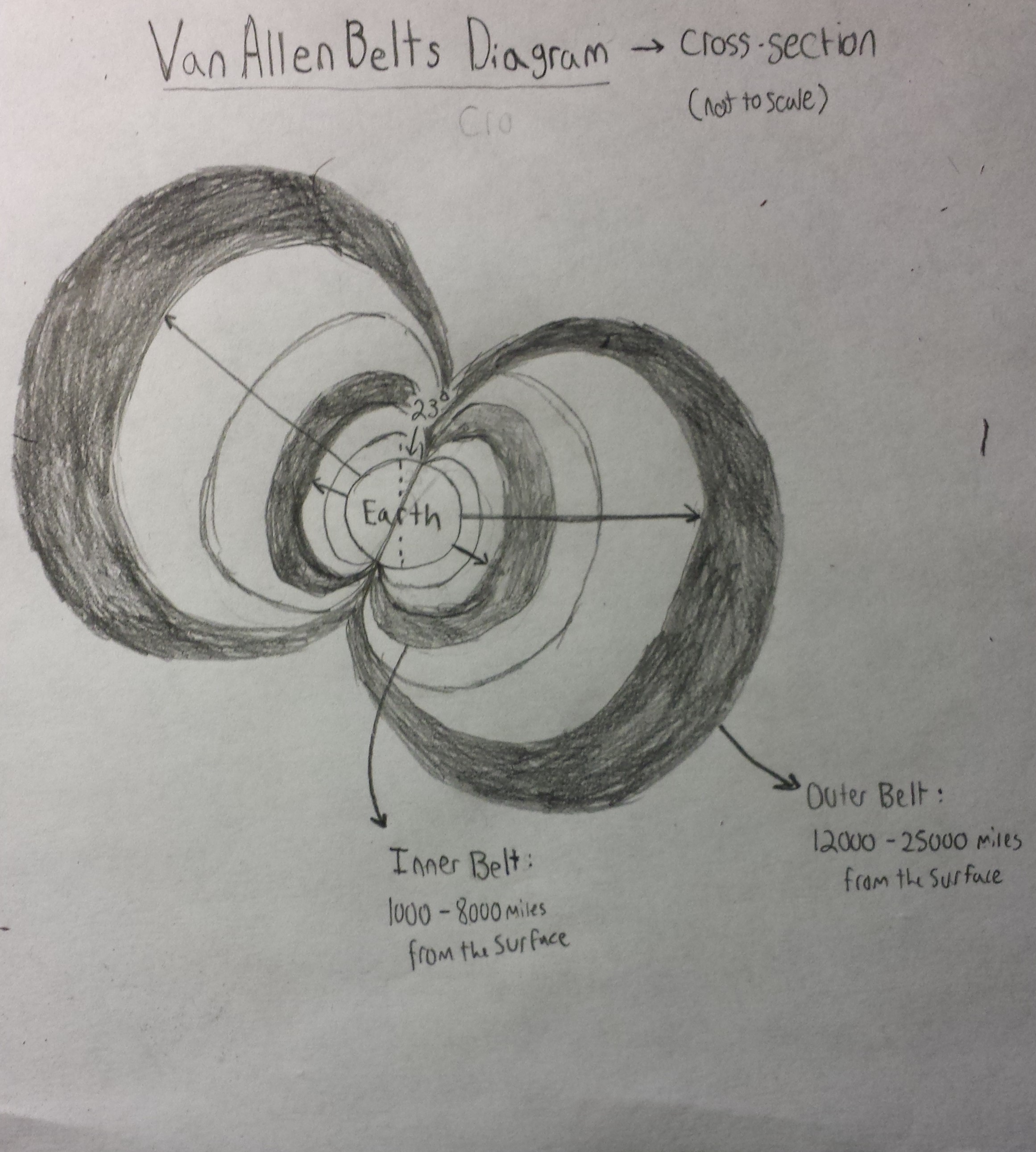
Cross-Section of the Van Allen Belts
The particles of these regions include fast moving electrons,and ions from the solar wind along with protons and other remnants of cosmic ray interactions with our atmosphere. All of these particles are electrically charged and thus their motion becomes highly constrained as they pass through our magnetic field; or magnetosphere. As they interact with our magnetic field lines, a force is exerted and influences their direction of motion. It attempts to make the particles rotate about the lines rather than allowing them to continue drifting in a straight line. Thus “sliding” begins to occur; the particles gain a spiral trajectory during which they orbit the field lines while vertically moving along them. Since the magnetic field is stronger as you get closer to Earth however the particles will stop and eventually reverse their motion as they approach the poles. This bouncing between the hemispheres establishes the permanent belts.
The constituent particles and stability of the belts however depends on the location.and thus the strength of the magnetic field. The inner belt is compact; ranging only from 1,700 km to 13,000 km above the Earth’s surface. It is made up primarily of high energy protons created during cosmic ray interactions with the atmosphere. Of the two belts, it is the most stable due to the higher magnitude of the magnetic field lines at that proximity to the Earth. While it gains high energy particles at a comparatively slow rate, it holds onto the particles for an extended period of time and reaches a much higher intensity than the other belt.
The outer belt ranges from 20,000 km to 40,000 km from the Earth’s surface and consists primarily of the ions and electrons that make up the solar wind. Due to the weaker magnetic field at that distance from Earth, the zone is tenuous and loses its particles very quickly. The constant supply of particles from the solar wind however means that the belt has plenty of material to be created from, though its dependence on solar wind particles means that its intensity fluctuates proportionally with solar wind activity. With this background information established, the information needed to created valid assumptions was gained.
2D Vector Fields:
Unfortunately, this also marks the point where my project strayed away from modeling the Van Allen Belts to a more general modeling of the Earth’s magnetic field. The initial task of modeling the magnetic field of the Earth was necessary to define the locations of the Belts with specific field lines that would be seen in the vector plot. Now with some research I found that the Earth’s field could be generally modeled as a magnetic dipole oriented with the south end pointed in the positive z direction. This model is a very basic assumption and ignores the effects of the solar wind on Earth’s magnetosphere, however the area where the Van Allen Belts are present does not get severely effected by these factors except in extreme circumstances. This means a model of a dipole will be generally accurate for our purposes. Thus the first task was to create a model of the magnetic field of the dipole.
The equation for the magnetic field of a dipole with respect to the radius was found to be
![\[ \vec{B_{dip}}(\vec{r})=\frac{(\mu_0)(m)}{(4\pi*r^3)}(2cos(\theta)\hat{r}+sin(\theta)\hat{\theta})\]](https://pages.vassar.edu/magnes/wp-content/ql-cache/quicklatex.com-3d217a43660c76323a7dd35189d6fa30_l3.png "Rendered by QuickLaTeX.com")
This equation was obtained from Griffiths’ Introduction to Electrodynamics. To insure the equation worked I began by applying a constant free version, evaluating only the variables. However, the equation was given in spherical coordinates which Mathematica can’t plot efficiently. To compound that issue, the command CoordinateTransform does not properly evaluate the points which led to several attempts to obtain the proper Cartesian conversion of our equation. Finally, I was able to find the command TransformedField which took into account the variables being used and allowed for a direct conversion. The code and direct conversion can be seen below.

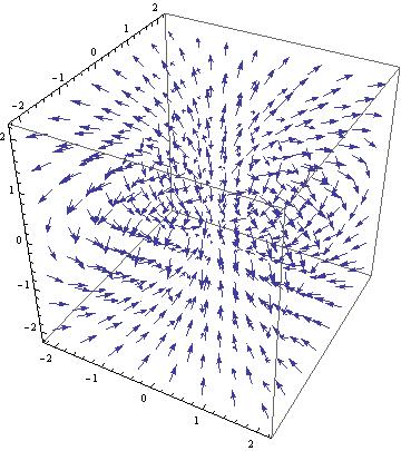
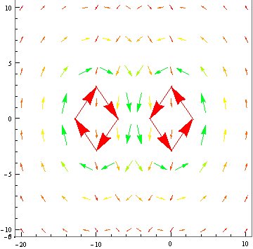
From these equations, I created a vector field of the xz plane with VectorPlot which can be seen below.
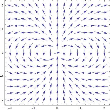
Simple vector model of the xz plane of the magnetic field of a dipole
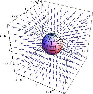
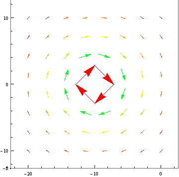
With this successful, I then applied the proper constants to the vector field components and attempted to recreated the field. These constants were the permeability of free space ( $\mu_0$ = $4\pi$*$10^{-7}$ $N$/$A^2$) and the magnetic dipole moment of the Earth ($m_{Earth}$ = $7.79$*$10^{22}$ $A*m^{2}$).The circle in the center of the graph represents the Earth, under the assumption that the Earth has a constant radius of $6.37*10^6$ m.
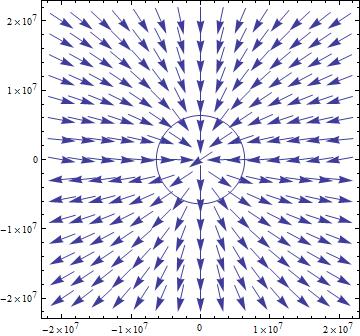
Model of the xz plane of the dipole’s magnetic field using Earth defined constants
Note that in this plot, the vectors seem to lack the fine structure of the previous field however the vectors are still properly oriented. They continue out from the southern hemisphere and seem to eventually loop back around and end in the northern hemisphere. I attempted a variety of scales and vector size values but no matter what, when the constants were applied to the equation they never had the same shape as the previous vector field. The other concerning aspect of the field was the fact that the vectors don’t seem to weaken as the field continues away from the Earth. It could be that the scale was just off so it was not evident, but even with the shifting of the scales, the vectors still seemed to remain the same size. The general direction and shape was obtained with these equations so I continued on to the next step.
3D Vector Fields:
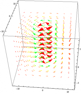
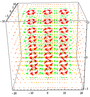
Applying the same methods as before, I used the vector field components from the obtained equation and using the command VectorPlot3D, I created a vector field of the general equation without the constants. This field can be seen below.
Simple vector model of the magnetic field of a dipole
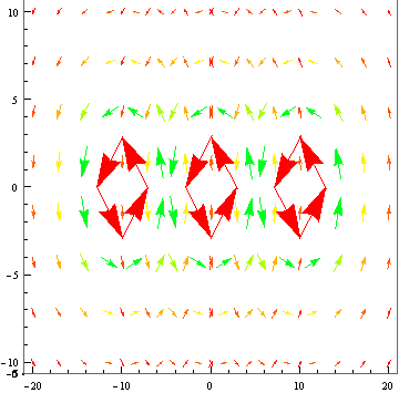
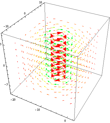
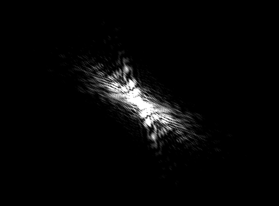
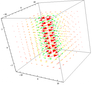
Without constants the shape of the vector field directly resembles the magnetic field of a dipole in 3 dimensions. Unfortunately, we also have the vectors not varying as expected as the distance from the origin increases. Regardless, after the success of obtaining the proper vector field shape and direction I decided to apply the proper constants to see if the shape would be altered as it was in the 2D graph. The constant applied vector field can be seen below. Once again the constants remain the same and the sphere in the center of the plot represents the Earth, assuming it is a sphere with a constant radius.
Vector model of the magnetic field of a dipole using Earth defined constants
As we can see, the same lack of detail is present when the constants are added to the vector field. However the shape and direction of the vector field are still generally correct though the fine structure is again lost. The vectors still don’t seem to vary with distance as well, which is troubling for actually plotting the field but the model does seem to accurately plot the field itself.
Further Plans:
Unfortunately it is at this point where I ran out of time and needed to call it quits on the project, with only the magnetic field of the dipole modeled. While I will discuss what I would have liked to change and go into more detail on complications within my “Conclusion”, I would like to take a moment to discuss where I wanted to continue on with this project. Specifically, next on the list would have been adjusting the vector field 23 degrees from the z-axis to account for the Earth’s natural tilt. I experimented with a few methods to do this but none of them were truly successful.
Next I would have liked to incorporate a model of the dynamo theory to account for the Earth’s magnetic field. One of the biggest assumptions made within this project was that the Earth’s magnetic field simply existed as a giant bar magnet in the surface. The magnetic field is actually generated by the motion of liquid iron present in the Earth’s outer core. Using this knowledge, I was hoping to create an animation that would allow the observer to alter the size of the planet and then the percent of the outer core took up of the interior. This would allow the observer to have a general model about how the magnetic fields change with different core sizes and thus the location of the Van Allen Belts. Knowing this, scientists could prep future scientific equipment for radiation exposure even if they needed to orbit within the Van Allen belts.
Here are my Mathematica Notebooks in case there were any questions on my code: 2D Vector Fields, 3D Vector Fields, and General Experimenting
Sources:
Griffiths, David, Introduction to Electrodynamics
Stern, David, Radiation Belts (http://www.phy6.org/Education/Iradbelt.html)
Dynamo Theory (https://courses.seas.harvard.edu/climate/eli/Courses/EPS281r/Sources/Earth-dynamo/1-Wikipedia-Dynamo-theory.pdf)
Magnets and Electromagnetism (http://hyperphysics.phy-astr.gsu.edu/hbase/magnetic/elemag.html)


 [1]
[1]![\text{DSolve}\left[\frac{\text{Current}(t)}{\text{Capacitance}}+\text{Inductance} \text{Current}''(t)+\text{Resistance} \text{Current}'(t)=0,\text{Current}(t),t\right]](https://pages.vassar.edu/magnes/wp-content/ql-cache/quicklatex.com-edf43b2ac32669349aa6c8d04ba9e32e_l3.png "Rendered by QuickLaTeX.com") [2]
[2] [3]
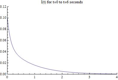
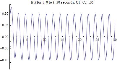
[3] . So, the initial current in the circuit must be 0.1 amps. Using a graphical guess-and-check method in Mathematica, I determined the value of the two constants to be approximately 0.05 each, resulting in a solution that is given by
 [4]
[4] [5]
[5] is the resonant angular frequency,
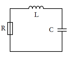
  is an initial value dependent on the voltage source, and t is the time. The inductance (L), resistance (R), and capacitance (C)are all determined by their respective circuit components, which are easily changed out for different ones.
  [6]
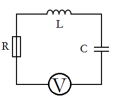
[6] ).
).![\text{DSolve}\left[\frac{\text{Current}(t)}{\text{Capacitance}}+\text{Inductance} \text{Current}''(t)+\text{Resistance} \text{Current}'(t)=E_{0} \omega \cos (\omega t),\text{Current}(t),t\right]](https://pages.vassar.edu/magnes/wp-content/ql-cache/quicklatex.com-4fd6cd2ab6f0ba47fdfaab15b71e9d9e_l3.png "Rendered by QuickLaTeX.com") [7]
[7] [8]
[8] [9]
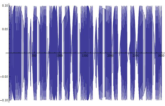
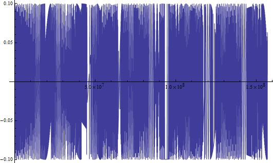
[9] . However, we can approximate the equation by only looking at the last term, which is a superposition of sin and cosine functions along with a couple exponential terms thrown in. The reason that we can apply this approximation is that the first two terms “damp out” quickly, and thus have exponentially less of an effect as time progresses. The reader may still be curious to see how much of an effect these terms have on the current flowing through the system: to that I say don’t worry! After my initial approximation, I will solve for these constants and compare the two cases.
 [10]
[10]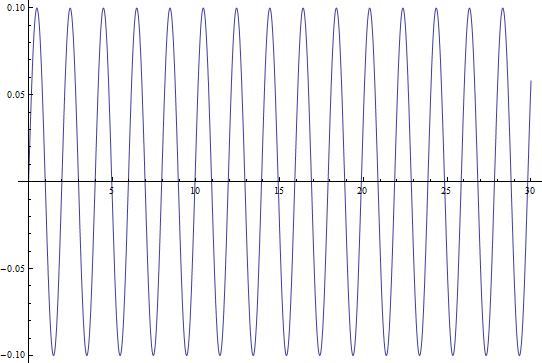
![C[1]](https://pages.vassar.edu/magnes/wp-content/ql-cache/quicklatex.com-86d57aecc373976151de585b5b2bec5a_l3.png "Rendered by QuickLaTeX.com") and
and ![C[2]](https://pages.vassar.edu/magnes/wp-content/ql-cache/quicklatex.com-12b2dbf736e307ece734ae42b09665aa_l3.png "Rendered by QuickLaTeX.com") and figure out graphically what they should be.
and figure out graphically what they should be. [12]
[12]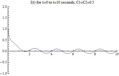
 [13]
[13]
 [14]
[14]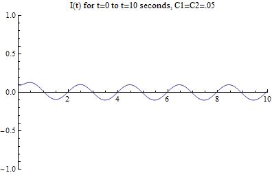


![\[ \oint \mathbf{B}\cdot dl=\mathbf{B}\oint dl=\mathbf{B}2\pi s=\mu_{0}I_{enc}=\mu_{0}I \]](https://pages.vassar.edu/magnes/wp-content/ql-cache/quicklatex.com-1863ee2b33a6f17c7d4c760c3efc98a9_l3.png "Rendered by QuickLaTeX.com")

 ,
,  and so we know that:
 . The magnetic field inside of the slab can found using Ampere’s Law again.
![\[ \oint \mathbf{B}\cdot dl=\mathbf{B}\oint dl=\mathbf{B}l=\mu_{0}I_{enc}=\mu_{0}IzJ \]](https://pages.vassar.edu/magnes/wp-content/ql-cache/quicklatex.com-7461b3b8e7706ef50752d43ae491c968_l3.png "Rendered by QuickLaTeX.com")

 , and so,
![\[ \mathbf{B(z)} = \frac{\mu_{0}I}{4\pi}\int \frac{dl}{\mathbf{r}^2}cos\theta \]](https://pages.vassar.edu/magnes/wp-content/ql-cache/quicklatex.com-849f8b8bdd2258e8d461601339a01f11_l3.png "Rendered by QuickLaTeX.com")
 is defined as the angle between the wire and our position vector
  . It follows then that