
In this post I will describing the specific charge distributions that I will be modeling and showing a brief derivation for the formulas I calculated.
Cylinder:
Problem 5.14 of Griffiths’ Introduction to Electrodynamics 4th edition describes a long cylindrical wire of radius a and steady uniform flowing current I over the outside surface of the cylinder. The magnetic field outside of the wire can be easily found by using Ampere’s Law.
![\[ \oint \mathbf{B}\cdot dl=\mathbf{B}\oint dl=\mathbf{B}2\pi s=\mu_{0}I_{enc}=\mu_{0}I \]](https://pages.vassar.edu/magnes/wp-content/ql-cache/quicklatex.com-1863ee2b33a6f17c7d4c760c3efc98a9_l3.png "Rendered by QuickLaTeX.com")
(1) 
When looking at points inside of the cylinder, or  ,
,  and so we know that:
(2) 
Combining our two cases in (1) and (2) we have:
(3) 
This is plotted below using Mathematica.
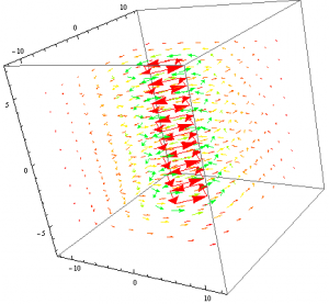
As expected, the magnetic field follows the commonly known right-hand-rule where the direction of the current curls around the direction of current.
Plane -> Slab :
Problem 5.15 of Griffiths’ Introduction to Electrodynamics 4th edition, a thick infinite slab extending from z=-a to z=a carries a uniform volume current  . The magnetic field inside of the slab can found using Ampere’s Law again.
![\[ \oint \mathbf{B}\cdot dl=\mathbf{B}\oint dl=\mathbf{B}l=\mu_{0}I_{enc}=\mu_{0}IzJ \]](https://pages.vassar.edu/magnes/wp-content/ql-cache/quicklatex.com-7461b3b8e7706ef50752d43ae491c968_l3.png "Rendered by QuickLaTeX.com")
(4) 
When looking at point outside of the slab, our  , and so,
(5) 
Sphere -> Ring:
After some research and individual work, I have come to realize that the magnetic field of either rotating conducting sphere or a spherical solenoid is very complicated. I decided to simplify the distribution to two dimensions rather than three for now. A sphere can be viewed as a collection of disks or rings, so I derived the formula for the magnetic field of a ring with radius R and steady current I .
By setting our coordinate system at the center of the ring, we know that the horizontal components of the magnetic field will cancel out through symmetry and the principle of superposition, and we are left with only the vertical component. This leaves us with:
![\[ \mathbf{B(z)} = \frac{\mu_{0}I}{4\pi}\int \frac{dl}{\mathbf{r}^2}cos\theta \]](https://pages.vassar.edu/magnes/wp-content/ql-cache/quicklatex.com-849f8b8bdd2258e8d461601339a01f11_l3.png "Rendered by QuickLaTeX.com")
where  is defined as the angle between the wire and our position vector
  . It follows then that
(6) 
References:
- Griffiths’ Introduction to Electrodynamics 4th edition
Mathematica Notebook:
https://drive.google.com/file/d/0B4ANWxS26h4FRE53d0d5aFRaN0U/edit?usp=sharing

Remember to put comments into your Mathematica code. Also, all work presented on the blog, including figures, must be your own. Please, take down the figure(s) that you did not produce.