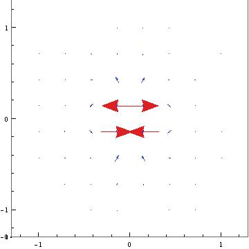
At the end of the preliminary data section, the Electric Field of a bar electret is stated to be approximately that of two opposing charged point charges at either end of the bar. However, little explanation is given as to why the bar can be modeled that way. If there was a justification given for this model, such as modeling many charges arranged in a line to show that the net fields cancel aside from the two charges at either end, the data would significantly benefit from this. Finally, it is unclear in the final data whether or not you are modeling a bar electret or an electric dipole.
Additionally, it is unclear why you chose the specifications for the dipole bar magnet, as well as the surrounding constants and values for the other scenarios. Although it is clear from a knowledgeable individual’s standpoint why the charges were assigned the equations as they were, a layperson may not be able to interpret the equations correctly. Additionally, including the full derivations for each scenario on the preliminary data in mathematica would streamline the analysis of the data significantly, as the constants themselves would become more clear with this. Additionally, the equations that yield the specific graphs in the final data you are showing should be wrote, so that I we can associate the data and figures easily.
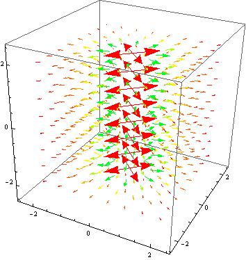
Finally, I suggest making the equations and derivations slightly more robust. By that I mean carrying out the derivations for these geometries in matter, as to better replicate the situations which a student may come across. Currently, this issue is approached without giving thought to the effects of polarization and the various materials involved. This may prove to both improve the depth and breadth of the project. Another concern that I have, although it may be a fault with mathematica, is that the field of the electret, does not show the field’s shape clearly. I suggest using a different graphing method, perhaps a contour graph, which would allow the interpretation of field lines much more intuitively. As such we would then expect the graph to take the shape of an imperfect dipole, as stated in your data.

![\[ \textbf{E} = \frac{q_e}{\epsilon_0 4 \pi r^2} \textbf{$\hat{r}$} \]](https://pages.vassar.edu/magnes/wp-content/ql-cache/quicklatex.com-3e809ffe305a5dd257991f875380bb3e_l3.png "Rendered by QuickLaTeX.com")
![\[ \textbf{E} = \frac{\rho R^2 }{2r\epsilon_0} \textbf{$\hat{r}$} \]](https://pages.vassar.edu/magnes/wp-content/ql-cache/quicklatex.com-555b4e970293d3e4e78338dd68259d29_l3.png "Rendered by QuickLaTeX.com")
![\[ V = \frac{p_o \cos(\theta)}{\epsilon_0 4 \pi r^2} \]](https://pages.vassar.edu/magnes/wp-content/ql-cache/quicklatex.com-e0d3b83684360e0a3e0cfeac94fc47a1_l3.png "Rendered by QuickLaTeX.com")
![\[ V = \frac{p \cos(\theta)}{r^2} \]](https://pages.vassar.edu/magnes/wp-content/ql-cache/quicklatex.com-17a8904c297439b92bb61b4fbb16897e_l3.png "Rendered by QuickLaTeX.com")
![\[ \textbf{E} = -\nabla V \]](https://pages.vassar.edu/magnes/wp-content/ql-cache/quicklatex.com-4af224d44a6a6606401ab97bc7cbea18_l3.png "Rendered by QuickLaTeX.com")

![\[ E(r)= \frac{1}{4\pi\epsilon_0} \int {\frac{\textbf{$\hat{r}$}}{r^2} dq \]](https://pages.vassar.edu/magnes/wp-content/ql-cache/quicklatex.com-3603622072e575c05df2ff882da37da9_l3.png "Rendered by QuickLaTeX.com")
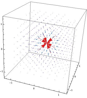
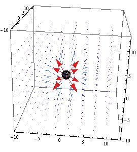
![\[ \oint _S {\textbf{E} \cdot d\textbf {a} = \frac{1}{\epsilon_0} q_e \]](https://pages.vassar.edu/magnes/wp-content/ql-cache/quicklatex.com-8686ebb11e96039929a6b5dd392fa8d8_l3.png "Rendered by QuickLaTeX.com")
![\[ \textbf{E}\ (4 \pi r^2) = \frac{1}{\epsilon_0} q_e \]](https://pages.vassar.edu/magnes/wp-content/ql-cache/quicklatex.com-6fe372d16c32971fe8a7d541237cc64f_l3.png "Rendered by QuickLaTeX.com")

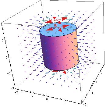
![\[ \textbf{E}\ (2 \pi r l) = \frac{1}{\epsilon_0} q_e \]](https://pages.vassar.edu/magnes/wp-content/ql-cache/quicklatex.com-0595b7d0f961955d35c5aac4f519ae28_l3.png "Rendered by QuickLaTeX.com")
![\[ \textbf{E}\ (2 \pi r l) = \frac{\rho\ \pi R^2 l}{\epsilon_0} \]](https://pages.vassar.edu/magnes/wp-content/ql-cache/quicklatex.com-f3e18ca089f99c71c53918df2c729a93_l3.png "Rendered by QuickLaTeX.com")
![\[ \textbf{E} = \frac{q}{\epsilon_0 4 \pi r^2} \textbf{$\hat{r}$} \]](https://pages.vassar.edu/magnes/wp-content/ql-cache/quicklatex.com-e3673892d325bdbcb5498bb574762e5a_l3.png "Rendered by QuickLaTeX.com")