
The brunt of my Mathematica work thus far can be found here: https://drive.google.com/file/d/0B0sdNVAIz9CjZkpLbnJEbTZjYXM/edit?usp=sharing
A rail gun is a simple assembly involving more complicated physics. It consists of a power supply connected to two parallel rails. Between these rails is a projectile that completes the circuit. The power supply (in this case we are modeling it as several capacitors) will release current into the circuit, instigating a number of forces which we will attempt to model. Below is a very generic
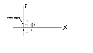
example of a rail gun circuit. Our original goal was to find the equations of motion for the railgun and hence functions for velocity and position. However, the mathematics required for this project has revealed itself to be immensely complicated, certainly much more so than we had expected. Many of the preliminary equations we find are based on the velocity itself, something we cannot know until the very end under our current plan. We have decided to go about it a different way, solving for all the relevant phenomena we had previously sought (current, b-field, emf) and using standard speeds of rail guns as constants to model said phenomena. In both our projects we will begin by deriving the most generic version of the magnetic field, caused by some current flowing through the circuit. This will require the Biot-Savart law:
(1) 
From Griffiths, the magnetic field at a point near a current carrying wire will be:
(2) 
Here, the magnetic field at a point p is a superposition of the magnetic fields created by the four sections of the current carrying wire. B1 and B3 will be the fields of the two rails, B2 will be the field of the projectile, and B4 will be the field of the power source.
(3) 
(4) 
(5) 
(6) 
The total field, of course, would be the superposition of these four equations. However, after having done a good amount of research and going through trial and error, we have discovered that when the rails (L) are much longer than the projectile and power source (d), we only need include the effects of the rails. Below is this magnetic field:
(7) 
Now, to find the magnetic field upon the projectile itself, we substitute L for x and get:
(8) 
From here, it is my responsibility to find out how the rail gun acts as a circuit. There are a couple parameters that I have been able to establish pretty easily. The first is the resistance of the circuit as a whole. This resistance is:
(9) 
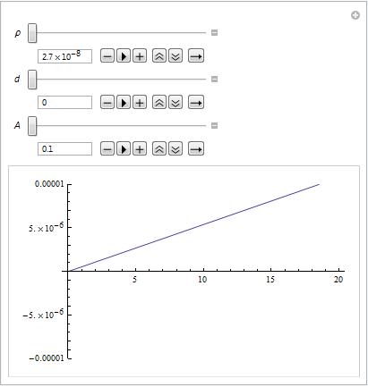
Where \rho is the resistivity and A is cross sectional area.
From there, we can start to look at the current created by the a capacitor with charge Q_0 and capacitance C discharging with the generic
(10) 
By replacing the R term we found above,
(11) 
We also know that this current is not the only current present in the circuit, as there is an induced current caused by the EMF created by the changing area and Magnetic Field (aka Magnetic Flux). We know that EMF ( \epsilon ) is equal to:
(12) 
We use the chain rule to say that:
(13) 
Where the second term
(14) 
Solving for the derivative of B with respect to L, I got that
(15) 
It is after this step where it gets complicated. I have used this expression to solve for EMF and then current, but the results are far from elegant and I am going to withhold them until I can validate the methodology. From here, there are two options. Griffiths proposes that EMF simply equals this result times velocity. However, I think that I may have to integrate the magnetic field over the area of the loop. I have tried this and have not had luck; the integral has been equal to 0 every time I’ve tried, something I know to be false. Once I figure this out, I will be able to animate and model all of these expression, and collaborate with John to achieve our final result.
As for our physical model, we will work with Professor Magnes to find something safer and more practical in the context of Vassar.
References:
Griffiths, David J. Introduction to Electrodynamics. Upper Saddle River, NJ: Prentice Hall, 1999. Print.
http://webphysics.davidson.edu/physlet_resources/bu_semester2/c11_RC.html
https://physics.le.ac.uk/journals/index.php/pst/article/viewFile/468/275

You need to make your file publicly available. Also, please take down any figures that were produced by you. All work on the blog must be your own original work.