The first item to be modeled will be the electric field of a sphere of uniform charge density. This will set the basic framework for any fields based off of a sphere.

To start, imagine a conducting solid sphere of some radius “R” that contains a total charge of Q. There are a couple of ways that the electric field of this configuration could be found. One is Coulomb’s Law, given by:

   

Where $ \epsilon_0 $ is the permittivity of free space and $ r $ is the separation between the source and the test.

The other (and far easier) is to use Gauss’s Law, given by:

   

Where $q_e$ is the enclosed charge of a Gaussian surface, $\textbf{E}$ is the electric field. Note that we are also taking a surface integral. All the math looks interesting, but what is a Gaussian surface? A Gaussian surface is an arbitrary surface at some distance from our actual surface (in this case our actual surface is the previously mentioned sphere), that matches the symmetry of the electric field generated by the object in question. What that means is that the electric field of our real object “flows” through the Gaussian surface in the same way it does the real object. Once this surface has been drawn we can use Gauss’s law to solve for the electric field of the object. In our case, the Gaussian surface is a sphere around out real sphere of some radius that is greater than $R$.

Now, because of symmetry, we can make a few nice simplifications. First, since the magnitude of the electric field is constant (the sphere is uniformly charged) $\textbf{E}$ can be taken outside of the integral, leaving the only thing inside to be $d\textbf {a}$. The integral of that is simply “A” but recall that this was a surface integral, so A is the surface area of our Gaussian surface, a sphere, which is simply $4 \pi r^2$.

Now all we have left is

   

Which is easily re-written as

   

and there is it. The electric field of a sphere (Griffith’s Example 2.2).

The electric field plotted 3D in mathematica:

Next, we’ll find the electric field of a cylinder of length L and radius R with a uniform volume charge density $\rho$. Again, it will be quite a bit easier to determine this using Gauss’s Law:

   

Just like the sphere we draw a surface that matches the symmetry of our object, and since we want the field outside the cylinder, we again choose a surface that has a radius greater than R, which I’ll call r.

Following the same line of reasoning as the sphere, the left side of the equation can be simplified to just the electric field, E, multiplied by the surface area of the surface. The surface area of a cylinder is given by $2\pi r l$ where $l$ is just the length of of Gaussian cylinder. This lets us write:

   

From here we need to find a way to express our charge enclosed. The definition of volume charge density is the total charge over the total volume, meaning that total charge is equal to charge density multiplied by the volume of the object. Again call our total charge Q and we know the volume of a cylinder to be $\pi r^2 l$. Taking our radius as R we can now write our Gauss’s law expression as:

   

Solving for $\textbf{E}$ yields:

   

Which is nicely plotted as:

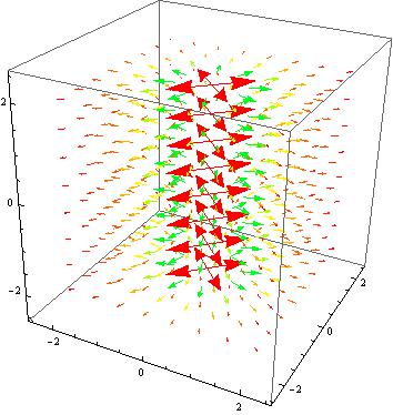
(excerpt from Griffith’s problem 2.16)

Finally, we have the electric field of a bar. The  electric field analogue to a bar magnet is whats known as a bar electret. For this type of model, we will assume that the electret’s shape is similar to the more common picture of a bar – that is that it’s length is much greater than its width.

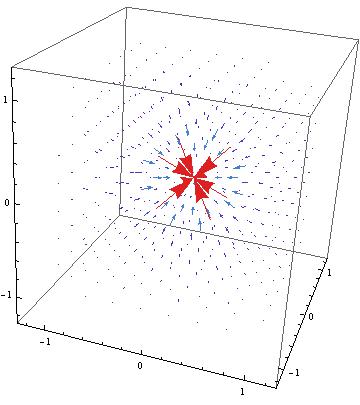
This electret requires us to use something other than Gauss’s Law. In this configuration the electric field is approximately that of two point charges of opposite charge. The electric field of a point charge is given by:

   

The plots shown below are of the two points of opposite charge.

      and

The mathematica code for these figures may be viewed here: Preliminary Data

 

Further modeling may show more complex systems build off of the ones shown here.