
Final Results:
The Matlab simulation of my final results. The PowerPoint Presentation associated with the simulation.
I have produced a simulation of the near and far fields of a two-element Yagi antenna. See the previously linked .m and .ppt files for a complete discussion of methodology and modeling.
Results:
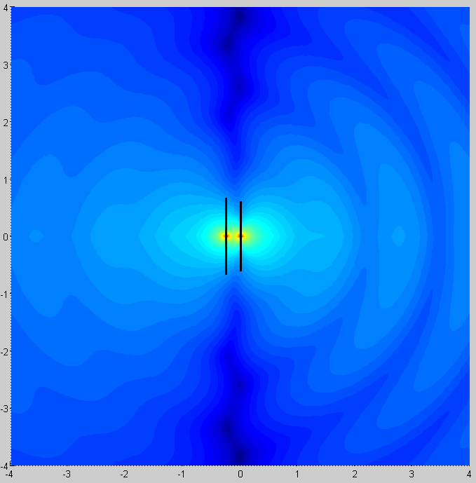
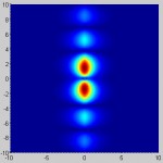
Figure 1: The calculated electric field strength(in dB) in the region surrounding the antenna. Antenna elements are shown to scale. Axis are in meters. Note the preferential transmission in one direction. An animated version of this plot is available in the linked Matlab file.
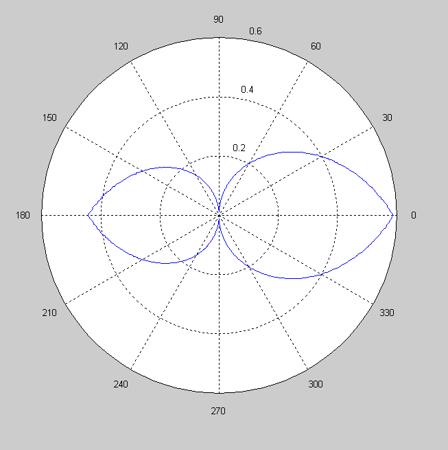
Figure 2: The calculated directivity of the antenna shown in figure 1. Note the similarity to the directivity plots show in previous entries for professional models of Yagi antenna.
——— 04/21/10 ————
Project Update: Yagi Antenna
Introduction
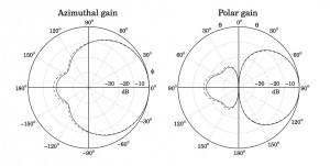
I am attempting to generate a visual representation of the EM fields produced by a directional Yagi-Uda antenna. I’ve used Yagi-Uda antenna for direction finding before, and I would like to know why arranging antenna elements like this:
Produces a directional gain pattern like this:
Yagi-Uda Antenna Background
All derivations presented here come from the text “Electromagnetic Waves and Antennas” by Sophocles J. Orfanidis, chapters 14, 21 and 22, or “Applied Electromegnetics” by Fawwaz T. Ulaby, chapter 9.
A Yagi-Uda antenna contains two types of elements: Driven and parasitic. Driven elements are conductors that are subject to an applied external AC potential source, such as an RF encoder or a function generator. Parasitic elements are left unconnected to any electrical components, and respond only to the incident EM fields of free space. When transmitting a signal, one element of a Yagi-Uda antenna is driven, while the rest remain parasitic. When receiving a signal, all the elements in the antenna remain parasitic, and the signal is measured as the voltage at the midpoint of the second longest element, as shown above. It should be noted that the directivity of a Yagi-Uda antenna is identical in both sending and receiving modes.
“Electromagnetic Waves and Antennas” presents a computation method for calculating the field produced by any arbitrary antenna configuration, driven by any arbitrary current. It is very long and involved, and I do not yet understand how to apply the method to a multiple element antenna. However, I can apply it to some simpler cases, such as a single element dipole antenna. I hope that by modeling the fields of the component parts of a Yagi-Uda antenna, I will eventually be able to assemble the information into my final answer.
Theory: Single Element dipole Antenna
With most antenna problems, it is easiest to formulate a solution if we are working, not with the fields, but with the retarded potentials, A(r,t) and V(r,t) . Recall that for a given charge distribution ρ, and a given current distribution J, the retarded potentials at point r are defined such that:
![]()
Where V represents all space where ρ and J are non-zero, and R is the distance between the potential source r’ and the point of interest r. Although most of our work will be done with potentials, recall that at any time, the fields E and B may be calculated from the potentials:
![]()
If we assume the potentials are driven by some harmonic source (as is the case with most radio applications), then the potentials will assume a harmonic time dependence:
![]()
Where k is the wave number, ω/c. Now let us assume a current distribution J for the antenna element of interest. Let us assume a thin dipole antenna on length (L) and radius (a) driven by a time dependant sinusoidal current source located at its midpoint. Assuming the dipole lies along the z-axis, and assuming the current must go to zero at the ends of the conductor, such a situation will produce the current distribution of:
![]()
Where the 2πa factor comes from the fact that the current will be distributed around the surface of the dipole. Evaluating the magnitude of A for such a current distribution and collecting all constants produces a potential:
![]()
Where θ is the azimuth angle. The key features to note here is that it produces a radial propagating wave with a 1/R falloff and a maximum at an angle broadside to the dipole:
For a periodic A, the magnitude of the E and B fields are proportional to the magnitude of A, so this plot may also be thought of as a plot of the magnitude of either E or B (though not both, as they differ by a phase constant).
My next step will be to see what happens to this field in the presence of multiple dipole elements, as well as model their response to an incident field at multiple angles.
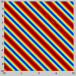
Incident EM waves at a 45 degree angle.
Note: All plots in this post were generated in Matlab. The .m file containing all the tools used to generate these plots is available in the previous post.
——— 04/21/10 ————
Here is a preliminary MATLAB simulation I have put together of my project. It contains a graphical display the fields of EM plane waves, as well as the fields generated by a dipole antenna, all time dependent. I will be assembling these into the fields of a Yagi-Uda antenna over the next 2 weeks.
——— 04/11/10 ————
I have found a technique online which allows for the computation of the fields induced inside an array of perfect conductors of an arbitrary shape when subject to a rapidly oscillating EM field. The technique makes a great deal of use of what is apparently known as the “Pocklington Integral Equation.”
I’ve also found the text “Electromagnetic Waves and Antennas” (the full text of which is available for download here). This text devotes two chapters to the application of the Pocklington Integral Equation for antenna of various shapes. I’m still working through the material, so I’m not sure if this method will lend itself to easy computation, but this is still the best lead I have so far at how to solve this problem.
——— 03/29/10 ————
My wave mathematica sheet can be found here.
Based on my experience with this worksheet, I am reconsidering my decision to complete my project with Mathematica. Mathematica seems to be great with number crunching, but clumsy and difficult to use when it comes to graphics. And since my project is about putting together a user friendly GRAPHICAL interface which can help with VISUALIZING a complicated EM field, I am starting to think that JAVA will produce better results than Mathematica.
——— 03/19/10 ————
Journal summary: Unfortunately, I have not found the journal to be especially useful or helpful.
If I have questions, I voice them in class or ask them during office hours; if I think of something important, I write it down in my class notes; if I find something interesting, I put it on the blog. The journal just seems to be redundant in light of these other media.
To date, I only have two entries in my journal. And they are both of the nature: “I don’t think I quite understand the concept of X. Why is this true?” And in both cases, the question I had was resolved in a later class.
——— 03/03/10 ————
Project: Yagi Antenna
I spent last summer at Dartmouth working with a team that launched high altitude balloons to study the upper atmosphere. The balloons would carry the payloads to ~90,000 feet and then burst, allowing the payloads to return to Earth under parachute, generally within 100 km of the launch site.
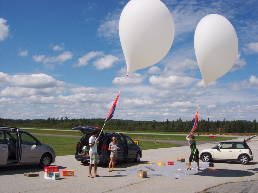
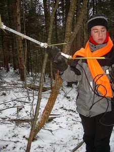
The payloads all contained onboard GPS receivers and radios which relayed their position back to us so we could keep track of their location. But we found that in the last 1000 feet of the payload’s descent, we would loose radio contact, and only be able to pinpoint the payloads’ landing location to within a few kilometers. Since the landing zone was usually in rough mountainous terrain and thick forrest, an uncertainty in the landing position of 1 km was too big to guarantee a recovery of the payload. We thus equipped each payload with a short range Emergency Location Transponder (ELT) and used a directional Yagi Antenna to home in onto the payload’s location after it had touched down.
[Image from RadioElectronic.com.]
Yagi antenna are a set of three or more parallel conductors, with their optimal dimensions and spacings determined by the wavelength of the radio signal the antenna is meant to receive. When arranged properly, the antenna will produce a very powerful response only when oriented towards the oncoming radio signal. There exist tables and manuals which give the proper dimensions for Yagi antenna at various frequencies, but I have no idea exactly WHY these dimensions should work for a given signal. As such, I intend to build a JAVA based program to simulate the response of a Yagi antenna in an oscillating EM field, and perhaps find a way to visualize exactly what the EM field is doing in the vicinity of a Yagi antenna to produce it’s directional behavior.
——— 02/16/10 ————
Mathematica analysis of refraction at a dielectric threshold can be found here.
——— 02/09/10 ————
My Mathematica solution to Griffiths 4.10 can be found here.
——— 02/01/10 ————
Proposed solution methods to Griffiths 4.1 part 2:
Method 1:
1) Assume the Hydrogen atom is composed of an electron held in “orbit” about a proton by electrical attraction, with orbital radius .5 Angstroms.
2) Calculate the “orbital” energy of the electron as if it were a point mass in a classical system. This is the ground state energy of the electron, (Eg).
3) Calculate the orbital radius associated with the orbital energy Eg+13.6 eV. This radius is the ionization radius (Ri).
4) As in part 1 of the problem, calculate the applied potential necessary to distort the hydrogen atom to (Ri).
Method 2: (Conceived by D. Bridgman-Packer)
1) Make a reasonable assumption for the dimensions of the plates (~ 1 cm^2 for example). Energy stored in a parallel plate capacitor (Ecap) can be calculated as:
Ecap = (C*V^2)/2
Where C= (EpsNaught*A/d)
2) Assume the stored energy is evenly distributed throughout the space between the plates (VolCap), so energy density as a function of applied voltage is:
Energy Density = Ecap/VolCap = (C*V^2)/(2*A*d) = ((EpsNaught*A/d)*V^2)/(2*A*d)
3) Calculate the applied voltage where the Energy Density exceeds 13.6 eV per cubic angstrom.
—————————————————-
A moving charge simulation referring to the first worksheet.
http://www.youtube.com/watch?v=eWaA9RiLsno
I would like to design a simple circuit to help aim a Yagi antenna. The big thing now in the game camera field is MMS cameras that send the pics to a cell phone. But, a lot of guys set up these cameras at considerable distance from the cell towers and then have a difficult time figuring out where to point the antenna.
What is the range of voltage produced at the antenna connector? This is generally a SMA connector for all game cameras I know about. I presume it is an AC signal at the frequency of the antenna (generally 850Mhz to 1900Mhz).
Could I put an analog voltmeter across the connector and get enough voltage boost with a two transistor Darlington circuit to be able to see a detectable swing on the meter’s pointer?
Thanks,
Mike Taylor
Katy Texas
Hi,
I have problem with the downloads. I am not able to open your matlab and mathematica files. Could you please help me.
With Regards,
Santosh
Jake: Noted. The current plots are in arbitrary units, so I didn’t bother to include any axis labels. I’ll make sure to include them for my final presentation.
Gabe: The ELT transmitter on the payloads was a 150 mW transmitter with a 1 meter dipole antenna transmitting on a 125.775 Mhz. While the payloads were in the air and in line of sight, the Yagi antenna shown above could pick up a signal from about 50 km. Once the payload was on the ground, the signal strength was diminished, and the detection range fell to around 10 km. I don’t know if that helps or not.
IDK if you can readily do this or not, but how weak of an em wave could your antenna pick up? I ask this because, you know, its relation to my project.
Hey Max, this looks like a great project with a practical purpose. My primary suggestion is for you to try to make a few of the graphs larger and thus more easily read. Also having labels and/or titles would just make it easier on the reader. I appreciate the pictures you had of yourself and others working on your project, it added an element of interest.
good luck!
“Note the energy associated with the groundstate of hydrogen is 13.6 eV.”
So it is. Fixed.
I like your description of solution paths. Note the energy associated with the groundstate of hydrogen is 13.6 eV.