Category Archives: diffraction

Conclusion: Diffraction Patterns of C. elegans

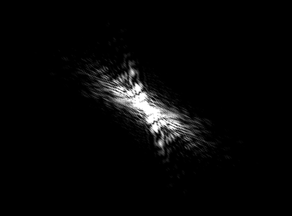
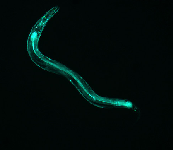
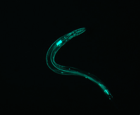
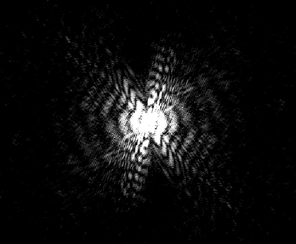
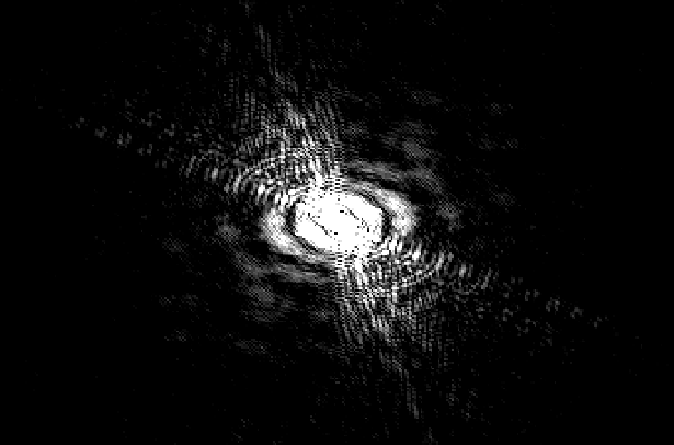
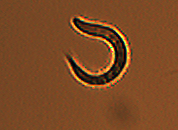
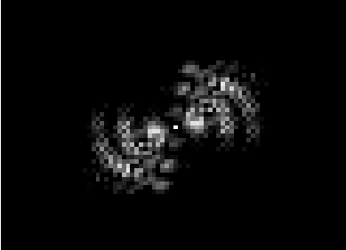
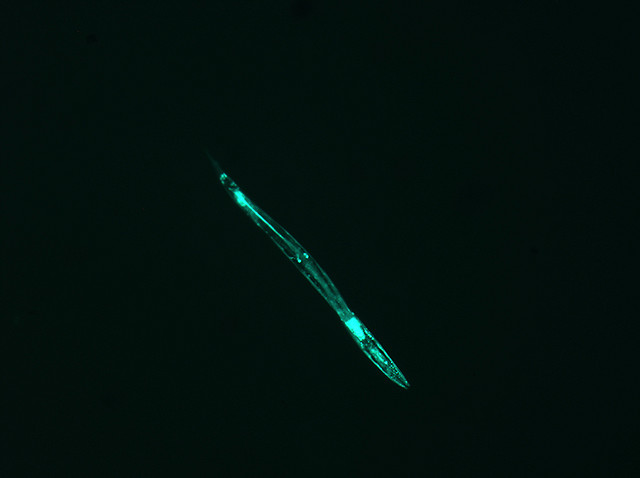
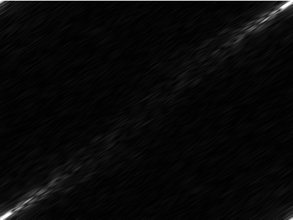
I set out to model the diffraction patterns created by C. elegans nematodes using mathematica, specifically using the diversely useful mathematical tool of the Discrete Fourier Transform. The Transform is a quick way to find the diffraction patterns from Fraunhofer diffraction and interference (far-field diffraction). In simpler language, $\left| FT^{2} \right|$ produces the diffraction pattern, which is an analysis of the Electric field strength across the aperture, in this case, the image. The goal of this project was to produce a “library” of shapes and their corresponding diffraction patterns. However, there were many obstacles that made it necessary for me to do quite a bit of relevant research.

When I started, I did not know that the type of diffraction I was studying was Fraunhofer. Diffraction patterns are a result of the type of wave and the type of experimental setup. In this case, the light source, the aperture, and the screen were are far enough away to classify it as far-field. Mathematically, $L>>\frac{b^{2}}{\lambda}=\frac{area. of. aperture}{\lambda}$ . The fact that this is an example of Fraunhofer Diffraction makes it possible to apply the FT (on Mathematica) to yield the diffraction pattern.

I came in with some preliminary knowledge of what Fourier Transforms were in theory. In general, when applied, it changes a function’s variable dependence: $F(t) \leftrightarrow \Phi (v)$. I did quite a bit of research on the derivations of the transform and understood the matrix calculations necessary to do the transform “by hand” (see Project Plan).

To produce good-quality images, it was also necessary to do quite a bit of exploring in the Mathematica Documentation Center, becoming familiar with a variety of image manipulation commands. Those included: sharpening, brightening, finding the pixel count and dimensions, cropping, changing the color scheme to grayscale, partitioning and reassembling images manually based on the pixel dimensions, and more, depending on what degree of manipulation the image needed.

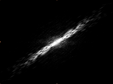
All in all, the images produced are not only pretty, but informative and now available for reference. Because it is mathematically impossible to go from the diffraction image to the shape, it is necessary to have some type of library, like the one I created, to go in that direction. (It is impossible to do it mathematically because when the Fourier Transform is applied, the phase information of the light is lost as the data is converted to the complex space.) Therefore, my “library” is useful because I have made it possible to guess the approximate shape and orientation of the worm from the diffraction pattern for some basic worm shapes. Another application for this analysis is that a compilation of several consecutive diffraction patterns shows the thrashing frequency of the worm. For example, if you took several pictures within a few seconds and found the diffraction patterns, the amount that the patterns change corresponds to the “thrashing frequency,” or the quantifiable amount that the worm wiggles.

If I were to continue this project, I would continue to build upon the library in the same manner, testing to see if different input image qualities would make a difference in the final product (if different pieces of the worms were fluorescing, if the worm was glowing a different color, etc). Finally, I would construct a real library (instead of this evolving blog site) that was easy to navigate, and generally more accessible for research.

Share

Final Data: Diffraction Patterns of C. elegans (revised)

Listed below are five sets of data (3-7), two images each. On the left is the photograph of the fluorescing worm. To the right is its corresponding diffraction pattern, produced with Mathematica.

First, a few comments:

Notice that each worm shape contains a different symmetry (or lack of symmetry). However, every diffraction pattern is symmetrical. The two images tend to share some symmetrical qualities, as noted below each image.

These diffraction patterns are due to the fluorescing parts of the worm (GFP, or green fluorescing protein). I believe that because of my image manipulation (converting to grayscale and brightening the image significantly), the diffraction pattern is approximately due to the entire worm and not just the fluorescing parts.

On that note, I’d like to discuss the parameters I used for image manipulation and Fourier Transforming.

  • The Fourier Parameters I chose were {0, 1} . These are the default parameters when using the FT command on Mathematica. I chose them among the three most common by ruling out the other two: {-1, 1} is used for data analysis (which I was not doing), and {1, -1} is used for signal processing (also irrelevant to my project). My choice of parameters specified the conventions I wanted the program to use when applying the transform.
  • The command ImageAdjust [image, {a, b}] adjusts the contrast of the image by a and the brightness by b. For most of my images, I adjusted the contrast by the same amount, but changed the brightness differently for each photo depending on my judgement.
  • I divided the images by hand and reassembled them according to the image dimensions, rectangles of dimension {col/2, row/2} (where col = the number of pixels in each column of the image, and row = the same for each row). I could have use the command RotateRight, but I did not figure that out until after I developed this equally effective algorithm.


IMAGE 3

Screen Shot 2014-04-24 at 12.22.33 PM Screen Shot 2014-04-24 at 12.50.08 PM   

This image has axial symmetry perpendicular to the axial symmetry of the worm. The worm is mostly linear, and so is the diffraction.

(complete file for image 3: book 3 )


IMAGE 4

3975048733_8abd2dce44_z Screen Shot 2014-04-24 at 1.11.07 PM

See comment for image 3.

(complete file for image 4: book 4 )


IMAGE 5

Screen Shot 2014-04-24 at 1.19.58 PM Screen Shot 2014-04-24 at 1.22.16 PM

Although this does not have an “inversion center” (the worm does not complete a loop), it is significantly less straight than the first few examples. Correspondingly, the diffraction pattern has an axial symmetry perpendicular to the “axis” of the worm. However, it splays out to a higher degree, indicating that the area of the pattern corresponds with the curvature of the worm.

(full file for image 5: book 5 )


IMAGE 6

Screen Shot 2014-04-24 at 4.10.28 PM Screen Shot 2014-04-25 at 8.51.20 PM

This further backs up my hypothesis from image 5. The curvature of the worm is great and the area of the pattern is also large. However, this worm does have a sort of “inversion center.” The diffraction image has an eye in the center, which is different than all of the preceding images. The curvature of the worm greatly effects the produced image, which is not surprising, but the overall shape of the image changes dramatically. With more circular worms, an “eye” is formed in the center of the diffraction pattern, and the pattern here has both some rotational symmetry and axial symmetry. With straighter worms, the diffraction is much more linear, containing only axial symmetry.

(full file for image 6: book 6 )


IMAGE 7

Screen Shot 2014-04-26 at 1.43.14 PM Screen Shot 2014-04-26 at 1.45.09 PM

See comment for image 6.

(full file for image 7: book 7 )

Share

Preliminary Results: C. elegans Diffraction Pattern Modeling

Staying true (so far) to my tentative project timeline, I acquired images of the C. elegans in various shapes, I have done quite a bit of research on Fourier Transforms and Fraunhofer Diffraction, and so far I have successfully transformed one image into the corresponding diffraction pattern.


IMAGE 1

sampleworm1I took this image and used Screen Shot 2014-04-21 at 5.16.08 PMmathematica to sharpen it –> setting it to grayscale and brighten it –> collect dimensional information –> apply a Fourier Transform, yielding (after some similar image manipulation):

This is a great diffraction pattern, but I had issues with the poor resolution and general image quality. To remedy this, I proceeded with images taken with a higher-resolution camera.

(full file for image 1: book 1 )

IMAGE 2

3975815904_e33a49b65b_z

This beautiful image needed some manipulation, similar to image 1: I converted it to grayscale –> brightened it significantly (to make it a more definite shape, and to get rid of the “holes” in the luminescing nematode)  –> collected image dimensions and data –> applied the FT. Unfortunately, I ran into a problem.

The produced image:

Screen Shot 2014-04-21 at 5.31.56 PM

Obviously this is quite different than the first diffraction image.

I had a few hypotheses:

1. The image was saved as a .jpg, but the same image was produced when I tried again with a .png version of the image.

2. The computer is phase- shifting the image so that instead of the origin lying in the center of the product, it is splitting the right side from the left side and lining them up in the wrong order. How can I rearrange and correct the phase shift in the output?

An analogy to the second hypothesis:

Screen Shot 2014-04-21 at 5.45.39 PM

Screen Shot 2014-04-21 at 5.45.53 PM


—>


It is as if, instead of centering the origin in the center of the produced diffraction pattern, the computer is putting the “origin” in a different place, and splitting the image, similar to the parabola I produced above.

My solution is a little underhanded. I divided the image into four equal rectangles, and manually rearranged them to produce what I knew was the true image:Screen Shot 2014-04-22 at 7.52.00 PM

(full file for image 2: book 2a  book 2b )

—————-

Reflection:

It is important to keep this process grounded: how is this relevant to Electromagnetism? The answer is that this entire process is only viable because of the laws of electromagnetism. I am analyzing the images by taking their Fourier Transforms. The diffraction pattern is the FT of the function that describes the electric field strength across the aperture of diffraction. In other words, I am applying an operation (the FT) to the image, which is a direct indication of the electric field strength across the aperture (the microscope slide) to mathematically find the diffraction pattern produced by the specific electric field array created by the shape of the worm.

Specifically, the diffraction pattern here is the Fraunhofer Diffraction pattern, or “far-field” diffraction, which occurs when the distances between the screen, aperture, and light source are appropriately far $L>>\frac{b^{2}}{\lambda}$. Diffraction effects are an outcome of the type of light wave.

It is also essential to realize what information is lost in the computation of these diffraction patterns. I am taking a real image, applying a FT to it, squaring the absolute value of the result, and arriving in a complex space. This process loses the phase information of the light, and as a result, it is possible to go from the image to the diffraction pattern, but impossible to find the image from the FT diffraction image.

Share

Project Proposal: Diffraction Symmetries of C. elegans

The C. elegans nematode is a common subject of biological studies, and has become more and more popular in physics research. I intend to find the diffraction patterns generated by the worms’ shape and log the findings into a Symmetries Library (with the eventual goal of using Group Theory to get the worm shape directly from a diffraction image).

The shape of the worm (photos to be taken with a microscope) will correspond to a particular diffraction pattern. I will model the Fraunhoufer diffraction patterns (Far-Field diffraction) of the electromagnetic waves (light waves) by generating images with Mathematica using the Fourier Transforms. The idea is that $\left | Fourier Transform | \right ^2 $ = the diffraction pattern. This project is a study of the behaviors of light waves.

I will eventually be keeping a log of my findings on the already existing website, the Diffraction Symmetries Library.

Share