
INTRODUCTION
For my project, I worked on the shot noise experiment and explained the concept of shot noise from a quantum mechanical perspective. The experimental component was necessary to understand how shot noise can be observed and measured. It was also necessary to model how transmission probabilities change with a changing voltage. The quantum mechanical component was necessary to describe an application of tunneling through step potential and its effects.
OVERVIEW OF SHOT NOISE
Noise can be observed when an electric current is generated from random independently generated electrons. Shot noise exists in certain macroscopic electric currents and can only be observed when the electric current is amplified thereby amplifying the noise. Shot noise is a result of the discreteness of electrons where the number of electrons arriving over a given period can be described using the Poisson distribution [3]. The randomly generated electrons create an uncertainty in the arrival of electrons. The standard deviation in the number of electrons arriving during that period is given by the square root of the number of electrons arriving for that period [3]. The statistical fluctuations in the arrival of electrons result in statistical fluctuations in the charge about its mean. These fluctuations are what we refer to as noise and can be observed through the shot noise experiment [3].
Fluctuating currents have also been theorized by Landauer [1] to result from random transmission of electrons from one terminal to another as individual electrons move across a potential barrier. The conductor can be modelled as N independent channels arranged in parallel to create the conducting wire [2]. In this case, each scatter-site can be thought of as a gap in the conductor. Electrons tunnelling through each independent channel, have a transmission probability Tn [2]. The transmission probabilities can be computed using the scattering matrix approach or by using Landauer’s formula.
This can be modelled as shown in Figure 1 below where electrons tunnel through the scatter site when moving from one terminal to the other. The wave packet tunnelling through the scattering site from the left of the scatter site to the right of the scatter site generates a current pulse. Electrons can tunnel from the right of the scatter site to the left of the scatter site, or vice-versa. The tunnelling of electrons is random resulting in fluctuating currents which we observe as noise [2].
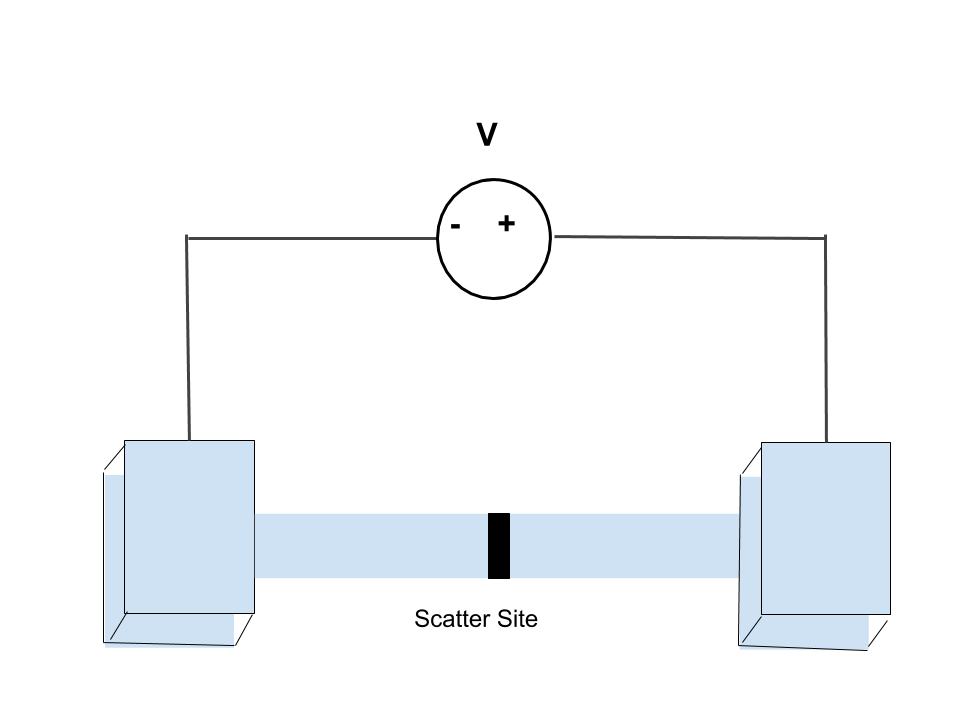
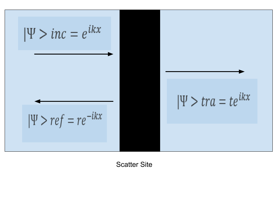
Figure1: a) Conducting wire modelled as a channel between two terminals with scattering sites through the channel b) Scatter site showing incident, reflected and transmitted wave functions for an electron approaching the scatter site from the left
METHODS
The shot noise experiment is set up as shown in the block diagram below. A photocurrent ejects statistically independent photoelectrons. The current is passed through a load resistor producing a dc voltage. In the low-level electronics (LLE), there is a high pass filter that passes frequencies above the cutoff frequency. The current is passed through an op-amp with a gain (G=100) in the preamplifier. The output of the pre-amplifier is then sent to the high-level electronics that includes a low pass filter and a gain (G=6000). The output from the HLE is an average amplified noise voltage. The frequency bandwidth that the high pass and low pass filter create determines the period over which statistically independent arrivals of electrons can be made. This amplified noise voltage can be calculated, and theoretical results compared to the experimental results.
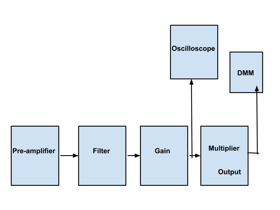
Figure 2: Block diagram for the shot noise experiment
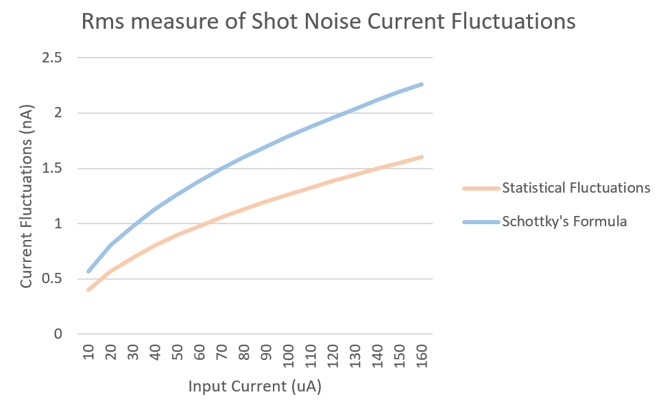
For this project, only the theoretical results were considered. An expression for the standard deviation in the current was used to calculate the rms measure of current fluctuations. These fluctuations were also calculated using Schottky’s formula (Eq 1). The two methods were used to compute the expected current fluctuation rms measurements [3].
![]()
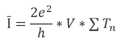
The model used to compute the expected current fluctuations was used to compute the sum of transmission probabilities of the N independent channels in the conductor. Landauer theorized that the time-averaged current can be computed from the conductance multiplied by the voltage and the sum of the transmission probabilities as shown in equation 3 below [1]. The sum of transmission probabilities was therefore calculated from the time-averaged current and the voltage using Eq 2.
RESULTS
Figure 3 below shows the results of the rms measure of the current fluctuations calculated using both Schottky’s formula and from the standard deviation in the current. From the graph below, the Schottky formula can be approximated as a suitable measure of shot noise current fluctuations as the current fluctuations are nearly equal. The average power transmitted by a noise source is proportional to the shot noise amplitude and is therefore proportional to the average dc current and to the as seen from Eq 1 and Figure 3 below. The average power is also proportional to the bandwidth frequency. Figure 4 below shows how the sum of transmission probabilities of n channels changes with changing voltage.
![]()
Figure 3: Rms measure of current fluctuations Figure 4: Transmission probabilities vs Voltage
DISCUSSION
The sum of transmission probabilities decreases exponentially with an increased voltage as seen in Figure 4 above. This corresponds to what we expect from Ohms Law and Landauer formula where conductance (1/R) increases with increased transmission probability, and conductance is inversely proportional to voltage. It, therefore, follows that transmission probability decreases with increased voltage. Another approach to computing transmission probabilities is through the use of the scattering matrix.
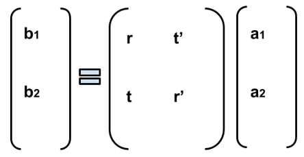
The scattering matrix has extensively been used to describe quantum transport by describing the relationship between electrons approaching a scatter site from the left and electrons approaching a scatter site from the right [2]. The wave equations for electrons approaching the scatter site from the right are similar to those shown in Figure 3 however the reflection and transmission coefficients r’ and t’ respectively [2]. The scattering matrix shown below is thereby necessary to calculate amplitudes of the waves approaching the scatter site from the left and those approaching the scatter site from the right. This offers an alternative way to compute transmission and reflection probabilities.
CONCLUSION
In conclusion, this study has found that fluctuations in an electric current can be attributed to the discreteness of electrons where we can use Schottky’s formula to calculate current fluctuations. It was also found that noise can be attributed to the uncertainty introduced by electrons tunnelling through a scattering site. The probabilities of transmission can be calculated using Landauer formula or could be found using the scattering matrix approach. The Schottky formula was found to closely match the count statistics approach to compute current fluctuations. It was also found that the sum of transmission probabilities decreased with increasing voltage.
REFERENCES
[1] Datta, S. (1995). Electronic transport in mesoscopic systems. Cambridge: Cambridge University Press.
[2] Lesovik, G. B., & Sadovskyy, I. A. (2011). Scattering matrix approach to the description of quantum electron transport. Physics-Uspekhi,54(10), 1007-1059. doi:10.3367/ufne.0181.201110b.1041
[3] Shot Noise Experimental Manual. NF Rev 1.0 9/1/2011. Vassar College
