Category Archives: Cedric

Magnetic Field Conclusions

When I started this project I initially had the intention to model the magnetic fields due to a cylinder, bar magnet, and sphere. Little did I realize that while I knew that these fields should look like theoretically, modelling them would  have been a great undertaking. The fields due to a bar magnet is that of a magnetic dipole and that in itself seemed as though it would have been a project. The sphere could have been modeled in two different ways: as a rotating sphere of charge, or a collection of current-carrying loops. Both were very difficult to find the magnetic field for at any given point and so I was at a loss for things to model.

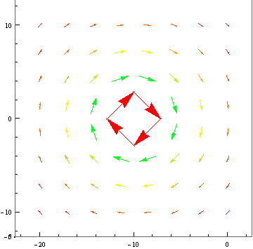
I was only able to successfully plot the magnetic field due to a line of charge rather than a cylinder since I was having trouble making Mathematica plot piecewise vector functions. The plot below was all that I had to work with.

1


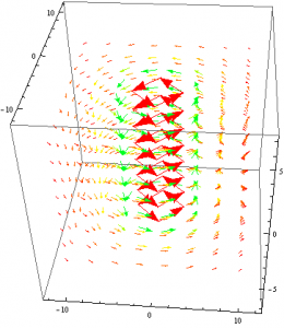
After some discussion with Professor Magnes, I decided I would take what I had, and make more complicated systems with it.

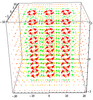
As seen in my previous Final Data post, I was able to show that if identical current-carrying wires were aligned next to each other, their resulting magnetic field would resemble that of the field due to a plane of current as the distance between them decreases. 

6

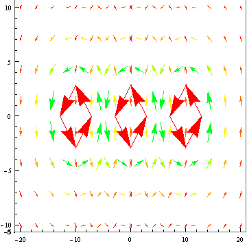
The only problem I faced was that I could not find a way to superimpose the vector fields from my aligned wires. While this would have made my model look nicer, it is still relatively clear to understand how the field lines add together.

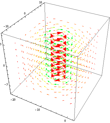
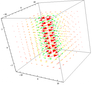
Next I decided I would use the same method that I used to mimic a plane of current and attempt to model a magnetic dipole. Rather than placing two identical current-carrying wires next to each other, I made one of them have a negative current. I would then plot their resulting vector fields and change the viewpoint such that only the x,y plane was seen.

7

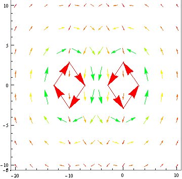
Again I was faced with the issue of superimposing my two vector fields. However, I suspect that if I found a function Mathematica that would do this for me, I would have indeed modeled a magnetic dipole.

While the topic of my project was by no means a very complicated one, it would be false to say that I did not learn anything from it. My understanding of how Mathematica functions as a program has grown and I have come to appreciate its capabilities. I also learned that while something may seem simple at first in theory, it can be very complicated to achieve in reality.


Share

Final Data

By using the formula for the magnetic field of a wire that I derived in my preliminary data,

(1)   \begin{equation*} \mathbf{B}(s) = \left\{ \begin{array}{lr} \frac{\mu_{0}I}{2\pi s}\widehat\theta & : s > a\\ 0 & : s < a \end{array} \right. \end{equation*}

I was able to model systems composed of current-carrying wires.

First I used the above equation and converted from Cylindrical to Cartesian coordinates. This was done because Mathematica will only plot vector fields in this form. I then plotted the resulting vector field due to a positive current.

1

This is exactly what we would expect to see for the magnetic field of current carrying wire as illustrated by the well known “Right-Hand-Rule”. The field lines are more intense towards the center of the of the wire while they decrease exponentially as they move further away. They are also oriented counter-clockwise since a positive current was used. Suppose now that we were to switch the current to a negative value.


2

As expected, the field lines behave in the same way as before expect they oriented in a clockwise fashion.

Below I changed the viewpoint of the magnetic field such that only the x,y plane is shown. This helps to visualize the field because the field does not change along the z-axis.


34

Now that I successfully found the Magnetic Field for a current-carrying-wire, I could make the system more complicated by adding additional wires.

Suppose that some identical wires were placed parallel to each other at some distance.

.5


Again I changed the viewpoint such that only the x,y plane is seen. 6

As you can see in the above plots, the fields in between the wires have a certain type of symmetry. The field lines point in opposite directions and as they get closer to the midpoint between the to wires, they are of the same magnitude and cancel. It is safe to assume that as the distance between the wires approaches 0, the magnetic field between the wires will no longer exist.
Above and below the set of wires, the direction of the field lines due to each wire is the same: +x below the wire and -x above the wire. Coincidentally, this shares similar traits to the magnetic field due to a plane of current; the field lines above and below the plane will point either in the positive or negative x direction while there is no magnetic field anywhere along the plane itself. This shows that a plane of current can be viewed as a collection of parallel wires with no distance between them.

Suppose now that I had two wires parallel to each other but rather than having both wires having the same current, they are opposite to each other.


7 

If Mathematica were able to superimpose the magnetic fields from the different wires, I suspect that the resulting field would resemble that of a magnetic dipole. However, I have not been able to find a function that will do this given two different vector fields and am limited by time to model a magnetic dipole using an alternative method. Nevertheless, the field that I was able to model does share some similarities to that of a dipole. The symmetry of the field lines are the same as those of a dipole. This is a result of two equal and opposite currents.

Mathematica Notebook

References:

  • Griffiths’ Introduction to Electrodynamics 4th edition


Share

Preliminary Data: Magnetic Field Modeling

In this post I will describing the specific charge distributions that I will be modeling and showing a brief derivation for the formulas I calculated.

Cylinder:

Problem 5.14 of Griffiths’ Introduction to Electrodynamics 4th edition describes a long cylindrical wire of radius a and steady uniform flowing current I over the outside surface of the cylinder. The magnetic field outside of the wire can be easily found by using Ampere’s Law.

    \[ \oint \mathbf{B}\cdot dl=\mathbf{B}\oint dl=\mathbf{B}2\pi s=\mu_{0}I_{enc}=\mu_{0}I \]

(1)   \begin{equation*} \mathbf{B}(s)=\frac{\mu_{0}I}{2\pi s}\widehat\theta& : s > a \end{equation*}

When looking at points inside of the cylinder, or s<a, I_{enc}=0 and so we know that:

(2)   \begin{equation*} \mathbf{B}(s)=0& : s < a \end{equation*}

Combining our two cases in (1) and (2) we have:

(3)   \begin{equation*} \mathbf{B}(s) = \left\{ \begin{array}{lr} \frac{\mu_{0}I}{2\pi s}\widehat\theta & : s > a\\ 0 & : s < a \end{array} \right. \end{equation*}

This is plotted below using Mathematica.

Cylinder

As expected, the magnetic field follows the commonly known right-hand-rule where the direction of the current curls around the direction of current.

Plane -> Slab :

Problem 5.15 of Griffiths’ Introduction to Electrodynamics 4th edition, a thick infinite slab extending from z=-a to z=a carries a uniform volume current \mathbf{J}=J\widehat x. The magnetic field inside of the slab can found using Ampere’s Law again.

    \[ \oint \mathbf{B}\cdot dl=\mathbf{B}\oint dl=\mathbf{B}l=\mu_{0}I_{enc}=\mu_{0}IzJ \]

(4)   \begin{equation*} \mathbf{B} = -\mu_{0}Jz\widehat y & : -a > z > a \end{equation*}

When looking at point outside of the slab, our I_{enc}=\mu_{0}IaJ, and so,

(5)   \begin{equation*} \mathbf{B} = \left\{ \begin{array}{lr} -\mu_{0}Ja\widehat y & : z > a\\ \mu_{0}Ja\widehat y & : z > -a \end{array} \right. \end{equation*}

Sphere -> Ring:

After some research and individual work, I have come to realize that the magnetic field of either rotating conducting sphere or a spherical solenoid is very complicated. I decided to simplify the distribution to two dimensions rather than three for now. A sphere can be viewed as a collection of disks or rings, so I derived the formula for the magnetic field of a ring with radius R and steady current .

By setting our coordinate system at the center of the ring, we know that the horizontal components of the magnetic field will cancel out through symmetry and the principle of superposition, and we are left with only the vertical component. This leaves us with:

    \[ \mathbf{B(z)} = \frac{\mu_{0}I}{4\pi}\int \frac{dl}{\mathbf{r}^2}cos\theta \]

where \theta is defined as the angle between the wire and our position vector \mathbf{r}. It follows then that

(6)   \begin{equation*} \mathbf{B(z)}=\frac{\mu_{0}I}{2}\frac{R^2}{(R^2+z^2)^{3/2}} \end{equation*}


References:

  • Griffiths’ Introduction to Electrodynamics 4th edition

Mathematica Notebook:
https://drive.google.com/file/d/0B4ANWxS26h4FRE53d0d5aFRaN0U/edit?usp=sharing

Share

Project Plan: Electric & Magnetic Field Modeling

Sources:

  • Introduction to Electrodynamics by David J. Griffiths, Fourth Edition: Chapter 5

Model:

I will be creating models of the magnetic fields of a bar magnet, sphere and a cylinder. Each of these fields will be first be derived for continuous distributions and then modeled on Mathematica using its Vector Field plot function in 2 and 3 dimensions. Time-permitting, I will also model the magnetic fields for distributions that are not continuous (perhaps with varying current densities dependent on space J(r)). Example systems can be found in Griffiths’ Introduction to Electrodynamics exercises.

Timeline:

April 7-April 14: Complete project proposal and begin derivations

April 14-April 21: Alter project proposal as needed and complete derivations

April 21- April 28: Post derivations and begin Mathematica modeling

April 28-May 5: Final Mathematica modeling and combination with Peter’s Modeling

Collaborators:

I will be working with Peter Florio, who will derive and model the electric fields of the same distributions. We plan to compare our results side-by-side to observe the similarities and differences between our models and to notice the parallels in our derivations.

Share

Project Proposal: Electric & Magnetic Field Modeling

For my project, I will work with Peter Florio to model the electric and magnetic fields of a bar magnet, sphere and cylinder. I will be looking at the magnetic fields of these distributions in 3-space and modeling their vector fields using Mathematica and Maxwell’s Equations. Problems given in David Griffiths’ Introduction to Electrodynamics will be used as specific examples of these kinds of charge distributions. My results will then be compared to the electric fields of the same distributions found by Peter.

Share