My Computational Physics final project models fluid flow by relying on the analogous relationship between Electric Potential and Velocity Potential as solved through Laplace’s Equation. I used the Gauss-Seidel Method to model velocity/electric field changes using vectors that correlate to changes in velocity/electric potential which depend on the points proximity to metal conductors/walls of pipes.

Background

Why Fluid Dynamics?

My interest in investigating Fluid Dynamics stemmed from a lecture given on campus in early February by Dr. Kristy Schlueter-Kuck, a Mechanical Engineer whose research focuses on the applications of coherent pattern recognition techniques to needed fields to aid in solving a variety of problems. One example of this showed the application of these techniques onto devices that aid in the study of ocean surface currents and allowed for more accurate modeling of fluid dynamics. I found this topic to be particularly fascinating since fluid dynamics is a type of mechanical physics that we do not have a chance to explore in our curriculum and for the simple fact that modeling invisible interactions is always a cool topic to explore.

Modeling Fluid Flow

In completing research about Fluid Dynamics, I gained a better understanding about the physics behind Fluid Flow and was able to study the relationship Fluid Velocity had to Laplace’s Equation and how Velocity Potential obeys this equation under ideal conditions.

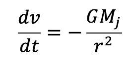
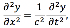
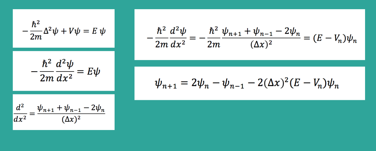
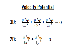
Laplace’s equation states that the sum of the second-order partial derivatives of a function, with respect to the Cartesian coordinates, equals zero:

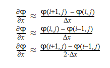
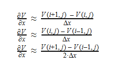
Using Laplace’s Equation, we can move toward solving for the Velocity Potential. In order to create the equation to solve for the Velocity Potential, we must first determine the first-order derivative of each function. The first derivative is essentially the change in potential with respect to the appropriate Cartesian coordinate, which in this case is x-coordinate. It can be written in a variety of ways as seen below:

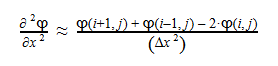
The second-derivative can be expressed as follows:

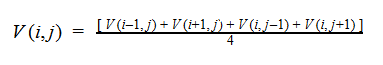
By plugging the second-derivative for each Cartesian coordinate into Laplace’s equation, we can find the equation to solve for the Velocity Potential. This equation can be simplified by assuming that delta_x=delta_y=delta_z. It tells us that the value of potential at any point is the average of its neighboring points.

In class, we studied Laplace’s Equation in Chapter 5 of the textbook as it applied to Electrostatic conditions where we were solving for Electric Potential and the Electric Field instead.

By solving for the Electric Potential in a similar fashion to how we solved for the Velocity Potential, we can see how these potentials are algebraically the same.

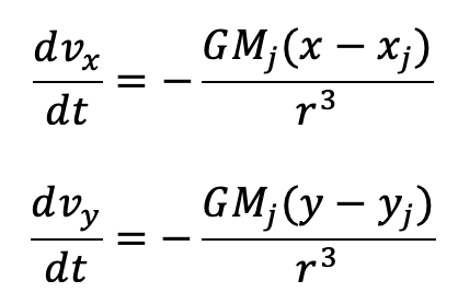
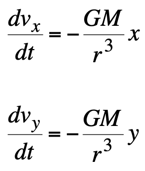
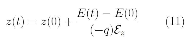
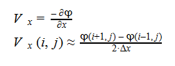
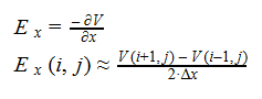
Additionally, we can find an analogous relationship between the negative derivative of each potential. The negative derivative value for the Electric and Velocity Potential for each Cartesian coordinate is equivalent to each respective component of the Electric Field and Velocity.

Since we know that both Velocity Potential and Electric Potential similarly obey Laplace’s Equation, and that there is an analogous relationship between Fluid Velocity and Electric Field, I thought it would be interesting to use this relationship to model Fluid Flow through the application of the Gauss-Seidel method, a method we also covered in Chapter 5 of our textbook. 

Gauss-Seidel Method

Chapter 5 teaches us about both the Jacobi and Gauss-Seidel Methods in the context of the Relaxation Method where both techniques allow us to computationally converge the potential at each point by averaging the surrounding values of its four neighbors, with the Gauss-Seidel storing the calculated values to inform further averages. We are able to use Laplace’s equation to solve for the potential at each point and utilize these methods to model the converging potentials, assuming we only know the boundary conditions.

By focusing on the Infinite Parallel Plates example and unpacking the mechanics behind each Method prior to the start of this project, I was able to achieve a better understanding of how the potentials were calculated and gained the tools to apply the Gauss-Seidel to more complicated scenarios.

Applications

My initial project proposal intended to explore fluid flow through the scenario of blood flow through veins in the body. I would have then explored cases that placed obstacles feigning pieces of cholesterol on the walls of the veins or some placed in direct path of the flow to model the impact these factors would have on the velocity vectors inside the vein. As my project developed, I realized that restraining my modeling scenarios around a singular vein/tube was limiting the amount of scenarios that the Gauss-Seidel Method could model, as well as under utilizing the analogous relationship between the Electric and Velocity Potential that I additionally had wanted to explore.

I then decided to recreate several of the Electric Potential/Electric Field cases demonstrated in the textbook and from there, analyze the figure and determine its analogous relationship to fluid flow. It is a direct way of making connections between the Electrostatic and Fluid Dynamic analogous relationship as supported by their reliance on Laplace’s Equation. Although it is not intuitive, both the Electric and Velocity Potential are solutions for Laplace’s Equations and therefore yield the same results under the same boundary conditions. I used figures solving for Electric Potential and Electric Field to inform me about the analogous relationship it holds to the Velocity Potential of fluid as well as the changing Velocity values due to the potential changes. I used my previous knowledge of how Electric Field vectors move from high to low potential to simulate fluid flow in pipes of varying geometry. In the last cases I modeled, I added blockages in an attempt to simulate more realistic scenarios for flow in the pipes.

Ultimately, my overall goal for this project has been multifaceted. I planned to investigate the physical phenomenon of Fluid flow and was able to do so by using Laplace’s Equation as the basis for an analogy between Velocity Potential (Fluid Dynamics) and Electric Potential (Electrostatics). I additionally utilized my previous knowledge about the Gauss-Seidel Method and its applications to Electrostatics to apply the method to Fluid Dynamics and gain a better understanding of the aforementioned relationship and its further applications.

Methods

To thoroughly explain my modeling process, I will walk through the steps I took to model     Case I: Infinite Parallel Plates/ Large Tunnel. I will showcase both approaches I took and explain some of the choices I made. This ground work allowed me to understand the applications of boundary conditions, how to input potential plates, and how to interpret the figures created and understand the physics behind the arrows and contour lines.

In order to apply the Gauss-Seidel method, I must first create a matrix of zeros. The nature of the Gauss-Seidel method requires us to know all values at all times. This is not merely an application that moves from through the matrix one at a time, we must know the potentials at all values to find the average at any point. Our matrix of zeros is our initial guess.

First Method:

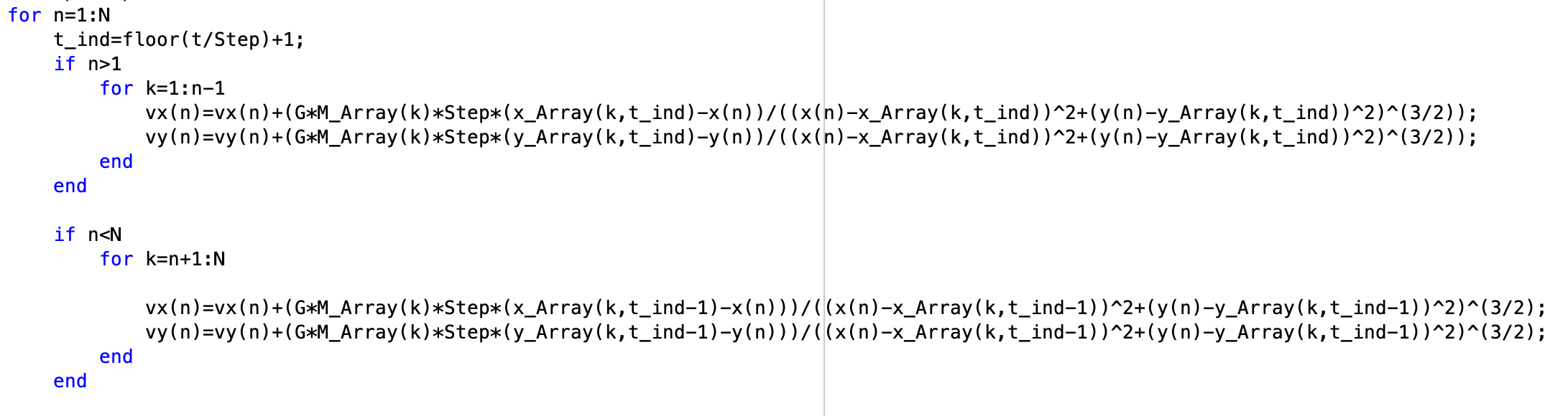
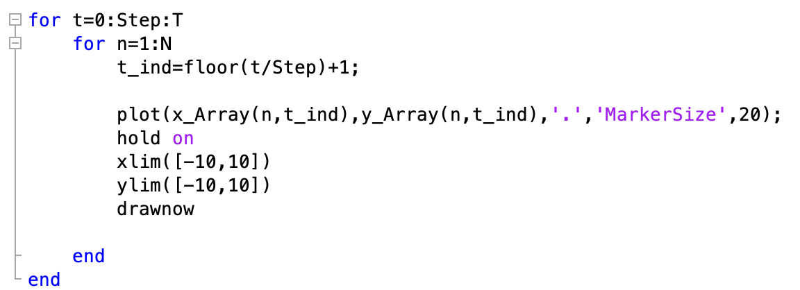
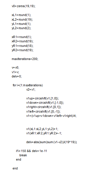
In my first attempt at creating this model, I wrote in the potential for each column between the two parallel plates. This didn’t leave much for the Gauss-Seidel Method to do. I created a for loop that ran 20 times, the maximum number of iterations I called for. DelV allows for the loop to break if the difference between average potential with each iteration, is smaller than the preset amount. I used a 2:6 range for i and j because if it were to start at (1,:) or (:,1), one of the points used in finding the potential average at that point would have a neighboring point of (0,:) or (:,0) which would cause an array error to occur. The for loop goes through all the potential positions for i and j, stores the potential average at each point into an array, and uses Laplace’s Equation to find the new potential average. The contour function plots the change in potential value (equipotential lines) while the quiver function inserts velocity vectors that correspond to the change in equipotential value. The Electric Field is determined using the gradient of the matrix values and the values of which are separated into two components.

Second Method:

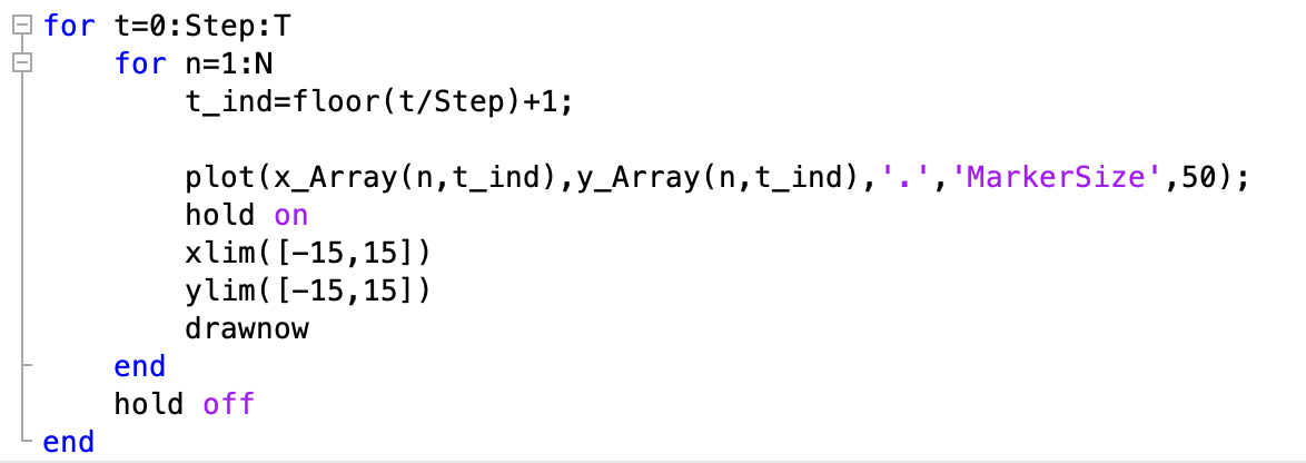
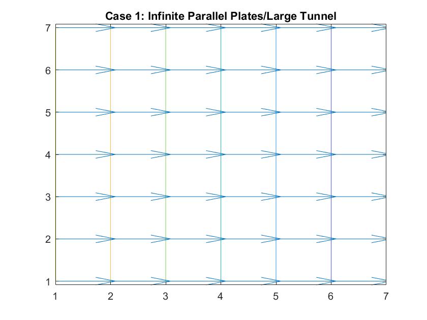
My second attempt at modeling the infinite parallel plates involved a different approach. In my initial conditions, I created each plate by giving its dimensions of length and width and location in the matrix. Inside the for loop I assigned a potential value to the section of the matrix where I had designated the plate to go. Placing it in the for loop ensured that it kept its value during every iteration, enforcing its boundary conditions. I solved for the potential similarly to my last attempt but did it in a way that did not involve going through i and j values individually. I instead accounted for shifts in position that allowed it to look at the neighboring potential values and use that to solve for the average at that point. I also now included an if statement that allowed the for loop to break if the difference between average potential with each iteration was smaller than the preset amount and the majority of iterations were completed. Though not in this image, I still used contour and quiver to model the equipotential lines and velocity vectors.

I found using the second method allowed me to have more control over the matrix in the more complicated models. Not having to figure out the number of i and j iterations that needed to take place for each case that called for different geometries allowed me to focus on playing around with the boundary conditions.

Results 

Summary

Part I: Fluid Flow (Over Objects / Drain)

• Case 1: Infinite Parallel Plates / Fluid Flow Through a Large Tunnel
• Case 2: Hollow Metallic Prism w/Solid, Metallic Inner Conductor / Fluid Pouring Down onto Raised Object
• Case 3: Two Finite Capacitor Plates / Fluid Coming Down onto Raised Object and then Draining
• Case 4: Two Infinitely Long Metal Sheets Crossed at Right Angles / Fluid Pouring Down onto Raised Object
• Case 5: Negatively Charged Inner Metal Conductor / Sink Drain Simulation

Part II: Fluid Flow in a Pipe

• Case 6: Two Finite Parallel Plates / Straight Pipe Flow
• Case 7: Two Finite Parallel Plates / Straight Pipe Flow w/blockage on Wall of Pipe
• Case 8: Two Finite Parallel Plates / Straight Pipe Flow w/ blockage in the middle of the Pipe
• Case 9: Curved Pipe or Electric Field through a Tube

_______________________________________________________________________________________________

Case 1: Infinite Parallel Plates / Fluid Flow Through a Large Tunnel

In the graph above, I modeled the behavior of the electric field between two infinitely long parallel plates using Method 1, which I described previously. The left plate had a potential value of 6 and the right plate had a value of -6. The equipotential lines represent where the potential is constant and they are always perpendicular to the electric field. The potential difference between equipotential lines is constant. We can see that the electric field is constant because of the equal distance between each line and because the arrow vectors are all the same length.

Analogous to fluid flow, in large tunnels, the flow is a steady, uniform stream, which is the ideal case to model. Here, the equipotential lines represent the velocity potentials and the arrows represent the velocity vectors of fluid flow.

This graph similarly models electric field/ flow fluid flow through a tunnel but utilized Method 2. I respectively set the potentials for each plate to 1 and -1 and allowed the Gauss-Seidel Method to fill in the potentials in between the plates.

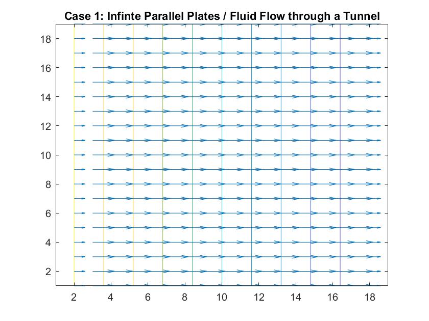
Case 2: Hollow Metallic Prism w/Solid, Metallic Inner Conductor / Fluid Pouring Down onto Raised Object

In the graph above, I modeled the behavior of the electric field around an inner conductor inside a box of neutral charge using Method 1. I set the conductor equal to a potential of 1 and the outer box equal to 0. I included an if statement in my code that prevented the for loop from reading the 1 values of the location in the matrix that represents the potential of the inner conductor when calculating the rest of the potential values of the matrix when using the Gauss-Seidel method. The distance between the equipotential lines represents the strength of the electric field, with the closer lines nearest to the inner conductor being where the electric field is strongest, which correlates to the longer vector sizes. The lines become further apart the further away we are from the conductor and the electric field weakens, but the potential energy is now converted to kinetic energy, which increases the further we go.

In terms of fluid flow, we can imagine the fluid continuously pouring down “into the page”, onto the object the center, which we can imagine is a raised platform and then pouring off the sides into drains at the edge of the box. The equipotential lines show the changing energy / velocity potential inside the fluid flow and the vectors indicate the direction of the fluid flow and the speed of the motion. It can also be described as a steady, uniform flow because even though the fluid is going in different directions, it is consistently and symmetrically flowing in these directions.

Case 3: Two Finite Capacitor Plates / Fluid Coming Down onto Raised Object and then Draining

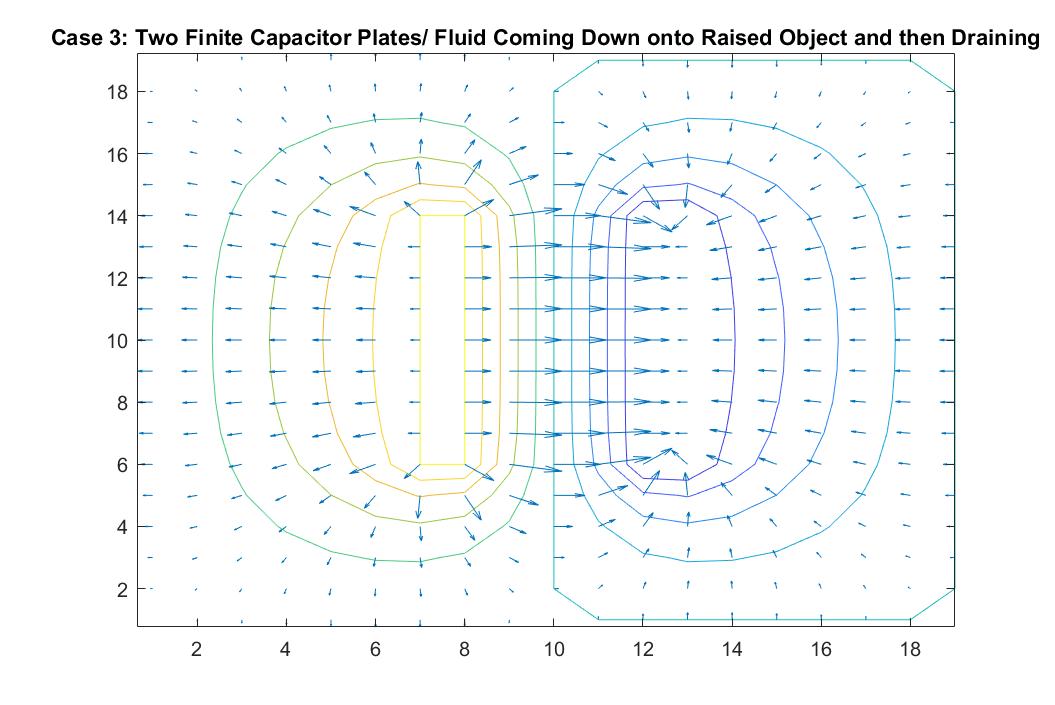
In the graph above, I modeled the behavior of the electric field between two finite parallel capacitor plates inside a neutral box using Method 2. I respectively set the potential values for each of the plates to 1 and -1, and reiterated the neutral boundary conditions of the box in the for loop. As expected, the behavior of the electric field vectors will move from the positive plate to the negative plate, with the electric field strongest in between the plates and with additional vectors pointing away from the positive plate and in toward the negative plate. The equipotential lines encircle each plate showing the highest potential values around the positive plate and the lowest around the negative plate. The electric field gets weaker the further it is from the plates as the distance between the equipotential lines increase. The darker color of these lines also correlate to the increase in kinetic energy.

This increase of kinetic energy goes hand in hand with the analogy to my scenario of fluid flow in this scenario. We can imagine the positive plate being a raised object and the negative plate acting as a rectangular drain. The direction of the velocity vectors would then inform us that the fluid that is being poured onto the object is cascading down in the right direction at a high speed into the drain (because of its longer vectors) and that the vectors pointing away from the raised platform are doing so because the fluid is cascading off of it outward, similar to Case 2. We can imagine the drain being a gradual decline, explaining why the velocity vectors grow in length as they grow closer to the drain.

Case 4: Two Infinitely Long Metal Sheets Crossed at Right Angles / Fluid Pouring Down onto Raised Object

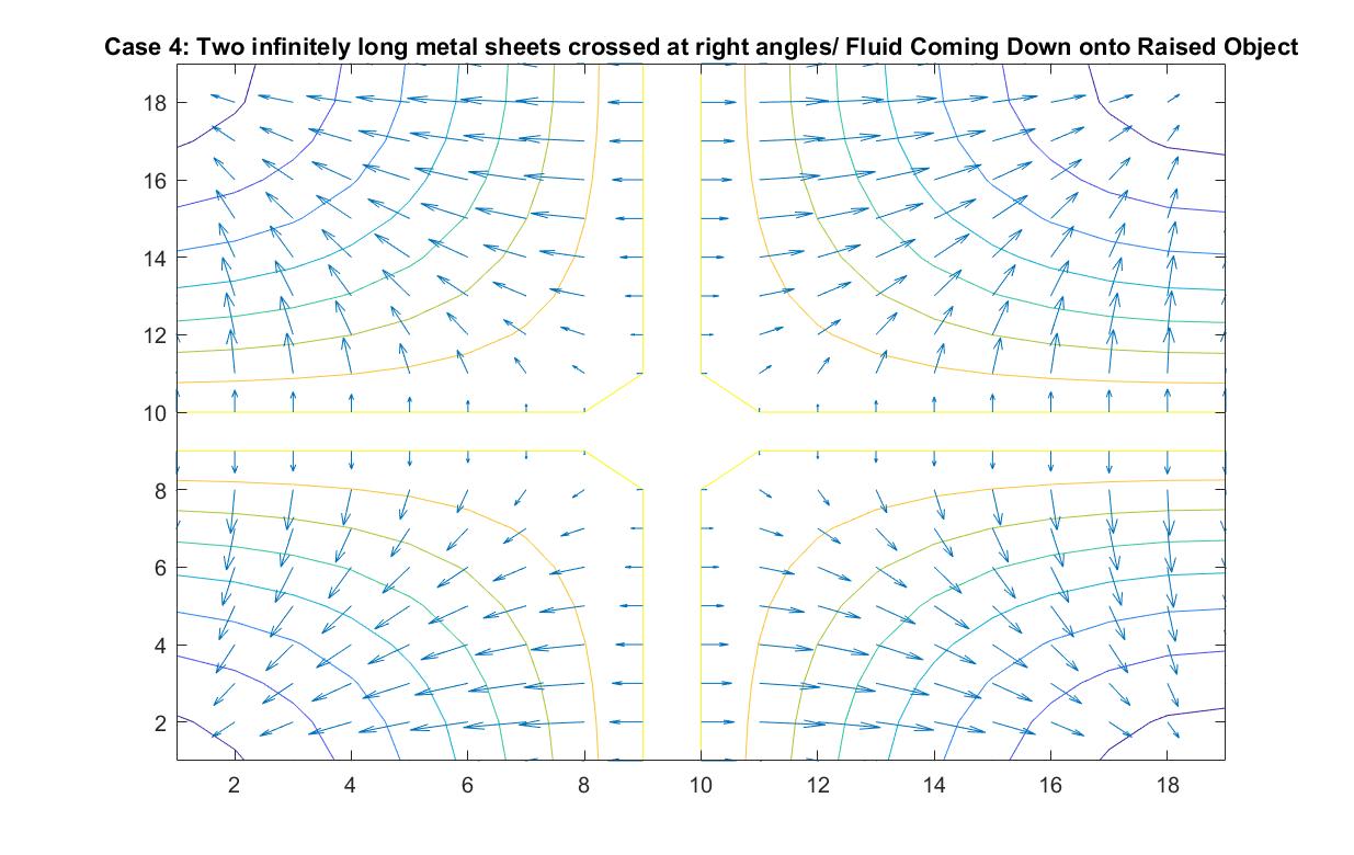
In the graph above, I modeled the behavior of the electric field around two infinitely long metal sheets crossed at right angles using Method 2. I set the potential energy value of both plates to 1 because I wanted to the electric field to point away from the sheets, anticipating the analogy I wanted to make to fluid flow.

In the scenario that the metal sheets are a raised cross-shaped object, the fluid ideally will flow down directly onto the cross and cascade down its sides into the concave area between the cross sections. The velocity vectors grow in length as the fluid motion speeds up due to its increase in kinetic energy when it flows down the decline at each of the four corners. The increasing distance between equipotential lines indicate that the electric field is getting weaker the further we get from the metal sheets or analogously that the velocity speed is starting to decrease in value the further it is from the initial cascading event at the raised platform.

Case 5: Negatively Charged Inner Metal Conductor / Sink Drain Simulation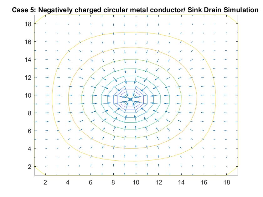

In the graph above, I modeled the behavior of the electric field around a negatively charged circular metal conductor inside a neutrally charged box using Method 2. I set the potential value of the inner conductor to -1 in order to manipulate the direction of the electric field and reiterated the boundary conditions in the for loop. As expected, the electric field grew stronger the closer it got to the conductor, as indicated by how the distances between the equipotential lines become increasingly closer. The electric field lines also grow in length indicating its strength.

Analogously, this behavior can simulate fluid going down a sink drain. Ideally, fluid flows down the curved decline of the sink into the drain at the center of the model, where the kinetic energy is at its peak and the velocity slowly increases as indicated by the growing vector length and smaller distances between velocity potential lines.

_______________________________________________________________________________________________

Case 6: Two Finite Parallel Plates / Straight Pipe Flow

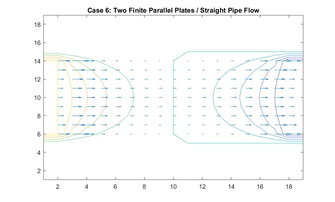
In the graph above, I modeled the behavior of the electric field between two finite parallel plates using Method 2 in order to analogously simulate fluid flow in a straight pipe. I also wanted to eventually model a curved pipe and used this model as an opportunity to build up to that. I used the potential differences between each end of the pipe to simulate the movement of the fluid inside the pipe. I set the left plate/end of the pipe equal to a potential value of 100 and the right plate/end of the pipe equal to a potential value of -100. I reinforced the neutral value of the walls. In comparison to the infinitely long parallel plates I modeled in Case 1, the equipotential lines curved at the ends of the pipe because of the zero potentials at the walls of the pipe. Rather than showing a constant velocity like the ideal model, the model shows a more realistic scenario where the velocity of the fluid flow is quickest at the center of the pipe and slowest the closer it is to the wall where the potential goes to zero. It makes sense to me that the velocity quickens as it reaches the other end of the pipe because of its increase in kinetic energy. This represents a steady, uniform flow.

Case 7: Two Finite Parallel Plates / Straight Pipe Flow w/blockage on Wall of Pipe

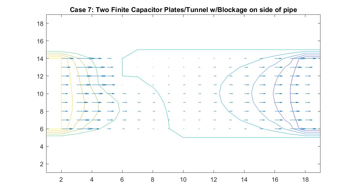
This model is similar to Case 6 but instead tests the behavior of the velocity vectors and velocity potential when there is an object placed on the wall of the pipe, causing a change in the width of the pipe. I utilized Method 2 and kept boundary conditions the same with the walls of the pipe having a potential of zero and having the potential values at the ends of the pipe be equal to 100 and -100. I added a square block with potential of zero to the wall of one of the pipes. I wanted it to be recognized as part of the wall so I set it to the same value as the pipe wall boundary.

The resulting model shows interesting equipotential lines. The long line that follows the edges of the pipe and then goes through the area where the blockage is is representative of a constant equipotential value that curves to show the effects of the non-uniform fluid flow. The equipotential lines are not as perfectly curved as in Case 6 on the left side of the tube because it takes into account the potential of the blockage.

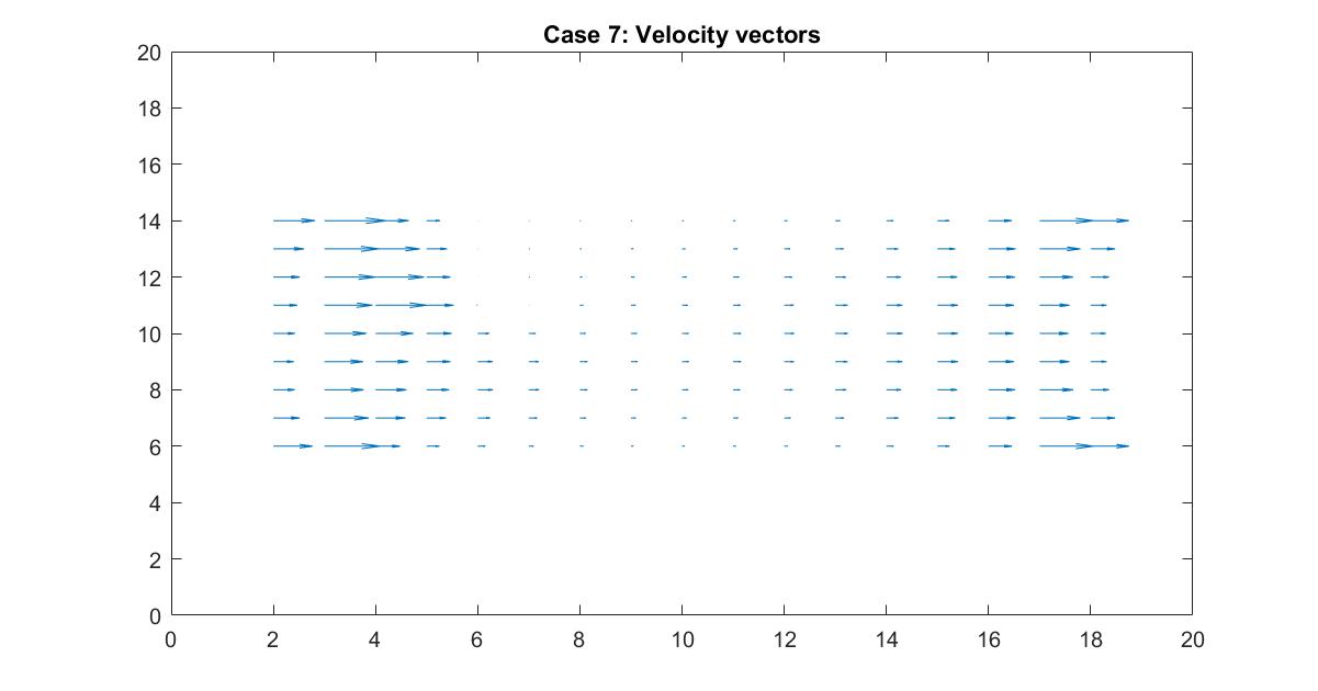
In the 2nd figure for Case 7, I isolated the velocity vector lines in order to highlight the behavior of velocity vectors around the blockage as they approached and moved away from it. Immediately to the right of the blockage there is a small velocity (short vector lines) because it isn’t in the direct path of the source of the flow whereas the left side of the blockage has high velocity (long vector lines) but stops suddenly because it has hit the object.

Case 8: Two Finite Parallel Plates / Straight Pipe Flow w/ blockage in the middle of the Pipe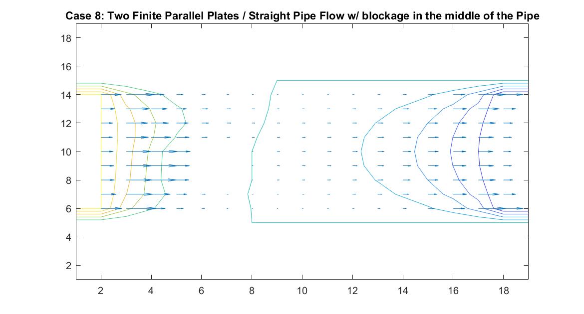

Like Case 7, this model tests the behavior of the velocity vectors and velocity potential by inserting an object inside the pipe but instead places it in the middle of the pipe in the direct path of the fluid flow. I utilized Method 2 and had the same boundary conditions as Case 6 for a straight pipe. I set the potential value of the blockage to zero and reiterated it in the for loop so the Gauss-Seidel Method would recognize the dip in potential value.

The resulting model is similar to Case 7 but because of the position change in the pipe, it has changed its effect on the equipotential lines. The blockage causes the equipotential lines on the left to move closer together and the velocity to increase. As first seen in the example of a straight pipe with no blockages, I set the left end potential equal to 1 and the right end equal to -1. Because of this, the fluid flow at the center of the pipe passes through the potential value of 0. In this example where we have the fluid reach potential values of zero sooner, since it encounters the blockage before the flow reaches the center of the pipe, we notice a faster drop in potential value.

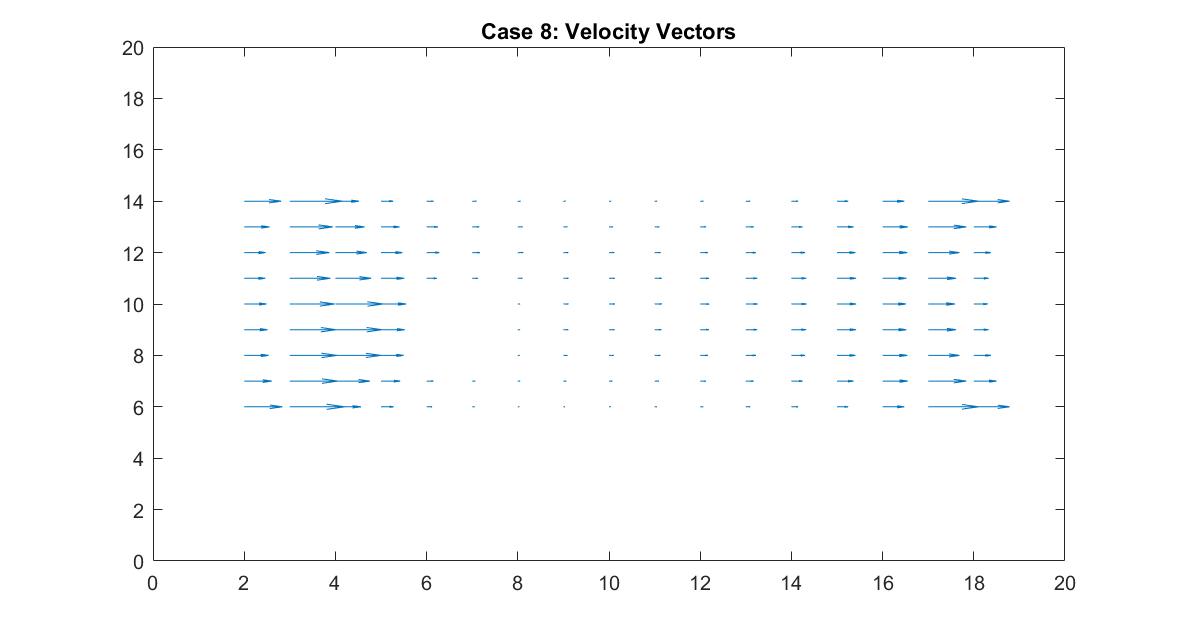
In the 2nd figure for Case 8, I isolated the velocity vector lines in order to highlight the behavior of velocity vectors around the blockage as they approached and moved away from it. It’s effect can only really be seen on the right side of the block where the velocity is much slower because it isn’t in direct path of the fluid flow.

Case 9:  Curved Pipe or Electric Field through a Tube

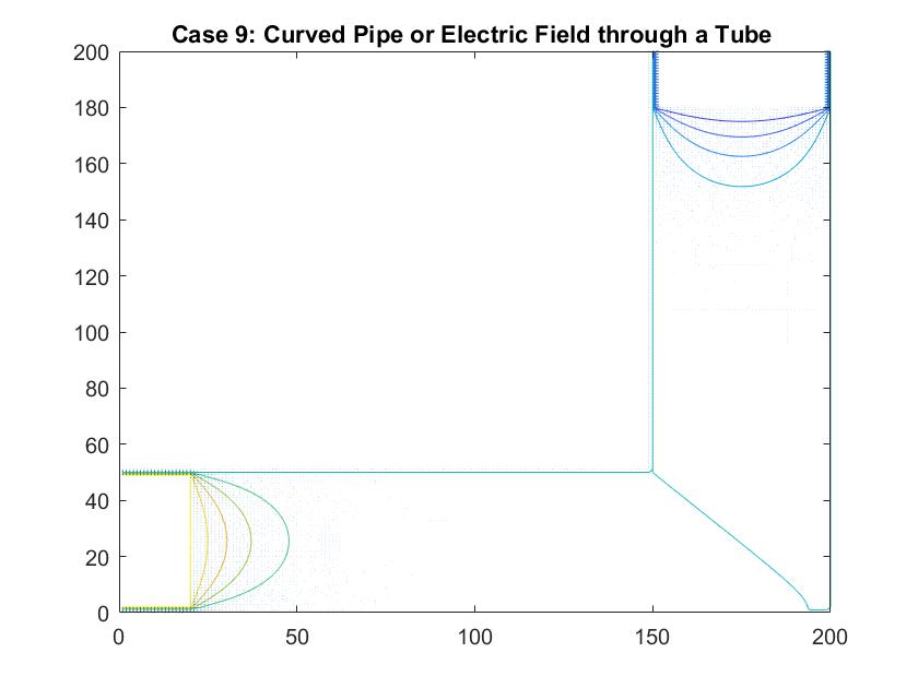
In the graph above I modeled fluid flow through a curved tube using differences in potential values at each end to facilitate movement. I utilized Method 2 of my Gauss-Seidel code to fill in the rest of the potential values inside the tube. I set the four walls of the tube equal to a potential of zero and the ends of the pipe to 100 and -100. There was a much larger cross section of the plot that I needed the Gauss-Seidel to ignore in calculating the potential inside the pipe. After testing out different values, I set the large area outside of the pipe equal to a potential of -10. I chose to do this because this value is relatively far from 0, which is the value for the boundary of the walls of the pipe. Similar to the straight pipe examples, the equipotential lines curve around the ends of the pipe, showing constant potential values. It makes sense that there is one equipotential line at the corner of the pipe at the curve because of the symmetry of the pipe.

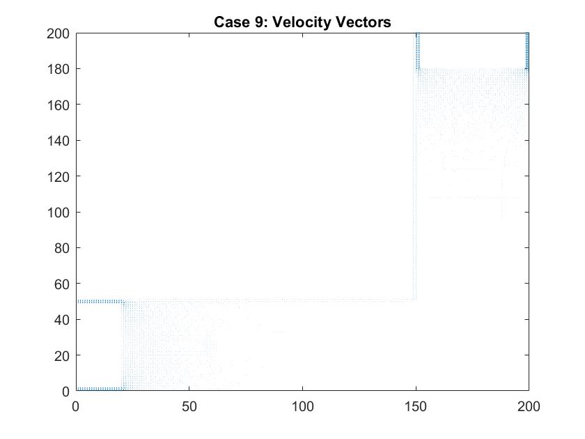
In a second figure for Case 9, I isolated the velocity vectors of the fluid flow to highlight the changes in the density of the arrows. Since the dimensions of this plot is much bigger than my previous models of the straight pipe, it is hard to see the differences in the lengths of the velocity vectors. We can assume that areas where there is a larger density of arrows, that there are higher magnitudes of velocity there. Here, they are found around each of the plates which follow the patterns we saw in the smaller scale straight pipe examples.

Conclusion

Through my work modeling fluid flow using analogies between the Velocity and Electric Potential, I was able to apply computational methods I learned in this course to equations we have been working with since Intro Physics as well as challenge myself through an immense amount of coding. Knowing the physics behind the scenarios that I was modeling and knowing what to expect in my results made debugging easier and made the project more rewarding. Also, getting into the practice of manipulating equations to explore different concepts, like how I used my knowledge of Laplace’s Equation and its applications to Electrostatics to explore a different type of Physics of which I had no prior knowledge in, Fluid Dynamics, was very useful.

One of the biggest limitations of my project had to have been the analogy I based this project on. The connection between Velocity and Electric Potential is not intuitive, especially since the way the electric potential is usually derived doesn’t make the relationship so obvious. Also, in modeling fluid flow, I assumed that the only kind of fluid flow is a steady stream without any influence of pressures and outside factors. It is never this perfect but this is something we understand since many models tend to first focus on the most ideal case, which I did for every scenario.

If I were to continue with this project and develop ways to further model Fluid Flow, I would explore other methods that could fill in the missing potentials between our known boundary conditions to see if there are more optimal/accurate ways to calculate them. Additionally, I would try to study the 3D case and create animations that could show the change in vector size as it would move through the simulation.

In this project, I focused on creating a program which would model the motion of any system of any number of objects interacting gravitationally. I used this project as a way to become more comfortable with computational methods we’ve already explored in class, to expand upon them, and to become more comfortable with the actual modeling and animation process, so that I can become more skilled in presenting the information I gather computationally. I was also attracted to this subject matter, because the generalized form I developed it for allows me to learn something new every time I plot it, exploring new systems every time.

Background

The “N-body problem” is one that has plagued physicists since Newton’s times. Newtonian/Classical gravity is defined by The behavior of two objects, interacting through Newtonian gravity, is well understood, easy to analyze by hand, and easy to model. However, as we increase the number of objects in our system, the problem immediately becomes far more complicated. People have studied the n-body problem for centuries, searching for a solution. In the late 19th century, the king of Sweden offered a prize to anyone who could find a general solution to the n-body problem. This challenge was left unmet, and the award went to Poincaré for an unrelated accomplishment. In more recent times, understanding the n-body problem has become far more feasible with technological advancements and the associated rise of computational physics. While there is no analytical solution to the n-body problem for 3 or more bodies, we can use computational methods to model and better understand gravitational interactions between celestial bodies and their resulting behavior.

We begin this analysis of gravitational interactions using the formula for gravitational force in conjunction with Newton’s Second Law.

From this, we getTo analyze this behavior, we must examine the system component by component. This results in the rate of change for velocity

This velocity rate of changes allow us to analyze the position of all of the celestial bodies in our system, since

Method

Equations of Motion

To model the n-body problem, I start by creating a set of input variables. This allows to me to create a very general program which should run whether we examine a system of 1 celestial body, 10, or 100. The program allows the input of number of bodies in the system, mass, initial position, initial speed, and initial direction of motion for each body. 

This is the code for collecting information from the user of the program. This excerpt of code applies to all objects other than the first.

Once the inputs have been obtained, we can proceed with the Euler-Cromer method to analyze the motions of however many bodies. 

The Euler-Cromer method uses a known rate of change for some desired variable, and adds the product of the rate of change with some step of the independent variable, to approximate some behavior. The distinction between the Euler-Cromer and Euler methods lies the fact that Euler-Cromer uses a newly calculated rate of change to calculate the new position. The Euler-Cromer method is effective for 2nd order differential equations, such as this case, where the Euler method fails. In the case of the n-body problem, this method takes the following form:

However, the above form only accounts for an object interacting with one other object. To address this, I summed the acceleration due to each object in my code.

This excerpt of code includes the summation of the gravitational forces and their influence on each object’s velocity.

Plotting/Animation

To understand how these interacting bodies behave, I examined their motion through graphing their paths and animating their motion. This plots demanded very little in terms of new plotting/animation methods, but rather demanded a lot of finessing, not all of which paid off. The drawnow command in conjunction with “hold on” and “hold off” produced the animation plots, whereas the same command only with “hold on” provided the plotted paths.

This is the code which plots the path of each object as we cycle through each time step.

Here is the code which plots the animation of each object’s motion. The primary difference between this code excerpt than the previous one is the use of “hold off”.

Results

It is hard to comprehensively discuss the results of this program because its input-based nature leaves infinite potential results. To examine how systems of n number of celestial bodies behave, I will discuss several cases as n increases.

Case 1:

This case is the most simple and best understood in case, in which two bodies interact gravitationally. The initial conditions of this case are as follows:

Graphing the path of each of these objects yields the following result:

Above is the path of each individual object in Case 1, on a plot in units AU.

This (messy) version of the previous plot is simply to provide clarity for each individual path of the objects.

Below is a clip of the animation for this case.

This is a 15 second clip of the animation of this case’s behavior. I could not include the entire animation because the video would not work, and GIFs are limited in length. If the animation is not playing automatically, click to view.

The results for Case 1 are precisely what one would expect from such a case. Object 1, the more massive object, experiences smaller acceleration due to the gravitational force from Object 2 than vice-versa, yielding a much smaller spiral of motion.

Case 2:

Maintaining the same conditions for the first two objects, we then consider adding a third into the system and see how it impacts the motion of the objects within the system. The initial conditions are as follows:

The results of Case 2 are graphed below.

The paths of gravitationally interacting objects 1,2, and 3 are shown above, on a graph of units AU.

This graph is simply the plot above, with sketched color coding to clarify the paths of individual objects.

An animation of this case is shown below:

This GIF is 15 second clip of the animation of Case 2. If not playing automatically, click to view.

Case 2’s results are less predictable than the results of Case 1, because of the additional object included. The most massive object (Object 1) still changes position the least, with each object of a lower mass moving more significantly than the last. This is the first case whose results we could not have calculated analytically. We can understand the trajectory of an object influenced by more than one object if one or more of those objects are held still, but the fact that each and every object experiences a gravitational force due to every other object eliminates the possibility of an analytical solution.

Case 3:

Adding a fourth body to our system, we will further examine how motion evolves as n increases. The initial conditions of this case are listed below. 

This case yields the following results:

On a plot with axis units AU, objects 1,2,3, and 4’s paths are shown.

The same plot as above is shown here with sketched on color-coding the clarify the paths of each individual object.

The animation for this case is shown below.

This GIF is a 15 second excerpt of the animation of Case 3. If it does not play automatically, click to view.

This case further demonstrates the transition from order in a two body system, to a far less ordered and less predictable system as n increases. Where in Case 1, object 1 moved in a clear spiral, here object 1 moves in a slow and oddly-shaped motion, as the forces it experiences are now based on the motion of 3 different objects.

From here we could continue to add more and more cases as n increases to watch this shift more clearly. However, while this program is theoretically general, and can run more than 4 objects at a time, as n increases, the program’s effectiveness decreases. The limitations and flaws in this program become and more likely to obstruct results, the more objects we consider in a system. I will discuss these flaws and the next steps to take to correct them below.

Obstacles/Limitations

1. 2-D
   The first limitation in this program is that it views celestial motion as 2 dimensional, where our universe is clearly exists within (at least) 3 dimensions. I made this choice to examine orbits and celestial motion from the perspective we usually view it ( we often view orbits as 2 dimensional, where they are not entirely), despite the fact that it does not entirely match reality.
2. Collisions
   One problem within this program is that it is not built to address collisions of celestial objects. When two objects wind up in the same position in the program– something that is physically impossible, but which this code does not explicitly prevent– they experience some large acceleration away from the other object. This behavior is not physically accurate and is a result of Matlab’s inability to understand an infinite acceleration.Here is an example of what a plot looks like when two objects collide:
   

   This plot (with axis unit AU) shows the way that objects react when they collide in this program. Both objects can be seen bolting away from one another immediately after their collision.

3. Inaccurate Plotted Points
   This is an issue that has not occurred often, but for which I have little explanation. Occasionally, in the middle of a program running, a new path of an unknown object will begin being plotted, which appears to be fairly massive, because it attracts the surrounding objects fairly strongly.
4. Path Plotting: Rainbow Everywhere
   As illustrated by my attempts to color-code my path plots, I have not yet found a way to plot the path of n number of objects in a for loop, where the program recognizes the paths of each object as distinct. This is why my original plots are all comprised of many colorful points, instead of a consistent color for each object. This problem also makes diagnosing the cause of the previous issue, because I cannot see which object the program is recognizing as also being in a different position.
5. Flashing Animation
   Assuming the links to the animations work properly, you can see that all objects except Object 1 are flashing. Having experimented with draw now, refresh data, hold on, and hold off, I have not yet identified a way to have a consistent, non-flashing animation of these systems’ behavior.

Where Next?

1. 3 dimensional
   Making this program 3-dimensional would be fairly simple upgrade to the program, to understand gravitational interactions as they actually occur in our universe. This would simply demand obtaining input information about the z component of motion, and applying it using the Euler Cromer method.
2. Conservation of Momentum
   Taking into account conservation of momentum would be one way to potentially address the limitation in my program in regards to collisions. Without significantly more information, this would likely demand the assumption of inelastic collisions in all cases. I could achieve this by adding the masses of colliding objects in one objects’ array information, and setting the other objects’ mass to zero. This however, may not actually be a large upgrade in terms of accuracy, as perfectly inelastic collisions are no where near the reality of what occurs when objects collide in space, so it would have its drawbacks as well.
3. Individual Track Paths of Different Objects
   Another clear next step would be to solve my issues in plotting, and develop a method where the program would recognize the individual paths of different objects, instead of considering every data point as unique. I admittedly am not sure how to accomplish this. However, once this is accomplished, it would play significant role in finding the error which causes random data points to pop up where they do not belong (problem #3 above).
4. Somehow Stop Flashing???
   The other significant next step in developing this program would be to solve the issue of flashing objects. This would likely just require even more deep diving on the internet into MatLab animation techniques, however the particular solution to this problem evaded me for the duration of the project length.

Another step moving forward that I would take with this program is to explore more explicitly what yields a stable (or stable-enough) orbit so that I could examine the behavior within a system of objects for a longer period of time. In this case, I would also explore more of the physics of the system, seeing how different objects’ velocities change with respect to time, how their acceleration changes, etcetera. With the program as it stands, exploring those would likely yield a fairly confusing set of graphs, with objects’ behaviors layered on top of each other in an incomprehensible mess. However, if I were to take the time to find systems for which this information is notable and readable, and sort through how to represent it sensibly, this would provide a lot more context for the behavior of these systems.

Project Outline

As a wannabe astronomer, I tend to make every possible project that I can about astronomy. It’s truly my passion. Orbital dynamics have always fascinated me and I’ve wondered the hypothetical solar systems where say Jupiter is even bigger than it is. Inspiration for this also comes from Exercise 16 in Chapter 4 of the textbook for the course that encourages the reader to examine the orbital dynamics of Earth and Jupiter when the latter increases in mass. So that’s what I decided to make this project about! In my project I use the Euler-Cromer computational method to ultimately produce simulated orbits of Earth and Jupiter, primarily to see how massive Jupiter must be to throw Earth out of its currently stable orbit around the Sun. I thought these to be interesting subjects since Earth is the planet that we live on and Jupiter is the most massive planet in the solar system, with fellow gas giant Saturn trailing far behind at about a quarter the mass of Jupiter.

What are the (astro)physics?

As a simulation of orbital dynamics, the physics at play here are gravitational forces. The differential equations of motion and position are easily derived from Newton’s 2nd law and some geometry. They are represented in their Cartesian component forms below:

When thinking of a computational method to use for solving differential equations, my mind flashed back to the beginning of the course when we started learning the Euler method and generally improved Euler-Cromer method. As with radioactive decay modeling, the Euler-Cromer method is more accurate at approximating the real curves than the Euler method is. This motivated me to elect the former as my computational method of choice for the project. The Euler method utilizes a for loop by simultaneously calculating new velocity and position values from their respective previous values and applying the change dictated by the differential equations. The Euler-Cromer method calculates the updated velocity values in the same way as the Euler method, but improves accuracy by calculating the updated position value using the recently updated velocity value, rather than the previous velocity value, as is the case in the Euler method.

Why 500 years?

On an astronomical timescale, where time lengths are generally billions of years, 500 years pass in not even the blink of the universe’s eye. However, there are several motivating reasons for this choice. First, the total time of the orbital simulation can be found by multiplying the number of iterations of the for loop by the size of the time step. In initial decisions, I wasn’t sure how to pick a valid value for either, but a place to start was thinking about the computational method I was looking to employ: the Euler-Cromer method. This computational method is valid for circular orbits, since the EC method creates a considerable amount of error at the point of perihelion, or when the planet reaches its maximum velocity. While the orbits of Jupiter and even Earth are eccentric, with eccentricities of 0.06487 and 0.00335 respectively, assuming circular orbits is not a very inaccurate approximation. For astronomical  background information, eccentricity is measured on a scale of 0 to 1, where e=0 is a perfectly circular orbit with the Sun at the exact center of that circular orbit.

For the Euler-Cromer method, I found scientific literature dedicated to investigating the limitations of different computational methods in mapping orbital simulations. The paper concludes that a time step of 10^-4 years or smaller is valid for EC. A time step of this size is equivalent to about 53 minutes. The effect of this is rather than producing a continuous circle of an infinite number of points, I approximate that through this method effectively as a discrete “circle’ of 9,917 points for Earth’s orbit and 117,633 points for Jupiter’s orbit. While a time step of 10^-4 years seemed suitable, the truncation error is proportional to the time step size squared, so I decided to test a time step of 10^-5 years to increase my accuracy by 100. The first issue was that decreasing step sizes causes the program to take longer to run. Additionally, if you don’t affect the number of points in the simulation as you decrease your time step by a factor of 10, then you also decrease the total time of the simulation by a factor of 10. This can obviously be balanced by increasing the number of points by an order of magnitude, which considerably increases the issue of a long computational time. Ultimately I decided to use the maximum valid time step of 10^-4 years because I felt as though the drawbacks to smaller step sizes heavily outweighed the minimal benefit in accuracy at that point.

Next, I had to decide on the (less important) value of the number of iterations for the loop. While a long run time wouldn’t be a terrible thing for other projects, in testing dozens of different mass values for Jupiter, I needed a shorter run time to be able to make steady progress even if it meant limiting the timescale of the simulation. I found a suitable run time when performing 5*10^6 iterations for a grand total of 10 million points (5 million for each planet’s orbit). Combined with my time step, this gives the total time of the simulation to be 500 years.

Important to confess here is that In the same scientific literature that I referred to when deciding an appropriate time step for the Euler-Cromer computational method, I discovered that while more accurate than the regular Euler method, the fourth order Runge-Kutta method is ideal for a simulation regarding orbital dynamics. While they conclude RK4 is considerably more accurate than EC without adjusting for step size, the Euler-Cromer method still is valid for the defined time step size regime. While I could have taken advantage of the increased accuracy of the Runge-Kutta method by utilizing a smaller step size to be able to increase total simulation time without a large cost to computational run time, I unfortunately found this out in the later stages of my project and didn’t feel as though I had enough time to start over.

The Simulation

In this simulation, I have assumed that all 3 objects, the Sun, the Earth, and Jupiter, are point masses. I have assumed the Sun to be fixed in place at the center of the solar system, and have allowed the Earth and Jupiter to move since that is exactly what I’m studying through this project. For the Sun, I use a mass value of 1.98847 * 10^30 kg, and for the Earth I use a value of 5.9722 * 10^24 kg. While Jupiter’s mass is 1.89813 * 10^27 kg, the project hinges on testing different mass values of Jupiter to see how it affects Earth’s orbit. I decided to set the mass of “Jupiter” to be an integer multiple of the Jovian mass, where “Jovian” is the term for things related to Jupiter. Here it is In a sentence: “Europa is a Jovian moon.” Thus, a “Jovian mass” is astronomical shorthand for “the mass of Jupiter.” As stated before, the simulation uses the Euler-Cromer method, with a time step, dt, of 10^-4 years, and a number of iterations, n, of 5*10^6. The planets are given their observed initial velocity values, both traveling counterclockwise.

The product of the simulation is a 2-dimensional (x-y) spatial mapping of Earth and Jupiter’s orbits. The axes of the plot are physical x and y positions. The length unit of the axes is the astronomical unit, AU. An AU is defined as the average distance from the center of the Sun to the center of the Earth, which is about 149.6 million kilometers. For the scale of orbits in the solar system, the AU is a very useful unit when compared to the kilometer.

Results

1 Jovian Mass

Mass of Planet = 1 Jovian Mass

Above is a simulation of the orbits of Earth and Jupiter where the mass of the Jovian planet is equivalent to 1 Jovian mass. This is the current state of our solar system, so this was mostly a check to see that the simulation was running correctly, as well as a way to have a result to compare future results to. The orbits remain completely circular and steady forever, with Earth staying at a distance of 1 AU and Jupiter staying at 5.2 AU, as expected.

10 Jovian Masses

Mass of Planet = 10 Jovian Masses

Above is a simulation where Jupiter’s mass is 10 times its standard value. There is almost no effect on Earth’s orbit here, so let’s increase the mass multiplier integer to 100.

100 Jovian Masses

Mass of Planet = 100 Jovian Masses

Here, the Jovian planet is now 100 times larger than it is in our standard solar system. While Earth’s orbit is beginning to be affected, the effect is minimal and causes a slight oscillation in the otherwise perfectly circular orbit. Important (and astonishing) to note is that in this case Jupiter is already more massive than the least massive stars that we have discovered, and under the right formation conditions, would actually be a second star in the simulation rather than a second planet. Less astonishing, is the realization that this minimal effect makes sense since the force of gravity is inversely proportional to the square of the distance between the two gravitationally interacting objects, the effects of the Sun overpower the effects of the farther away Jovian planet. Clearly, it’s going to take a lot of mass to really affect Earth’s orbit, so going forward lets continue to use increments of 100 Jovian masses.

200 Jovian Masses

Mass of Planet = 200 Jovian Masses

At a planetary mass of 200 Jovian masses, we can observe the oscillations deviating from a perfect, constant circle more than before. However, Earth is still very much attached to the Sun, so let’s keep going until it isn’t.

300 Jovian Masses

Mass of Planet = 300 Jovian Masses

At 300 Jovian masses, oscillatory motion is more pronounced than before.

400 Jovian Masses

Mass of Planet = 400 Jovian Masses

At 400 Jovian masses, Jupiter’s effect becomes more substantial.

500 Jovian Masses

Mass of Planet = 500 Jovian Masses

The trend continues for 500 Jovian masses.

600 Jovian Masses

Mass of Planet = 600 Jovian Masses

The trend continues for 600 Jovian masses.

700 Jovian Masses

Mass of Planet = 700 Jovian Masses

The trend continues for 700 Jovian masses.

800 Jovian Masses

Mass of Planet = 800 Jovian Masses

The trend continues (yes, still) for 800 Jovian masses.

900 Jovian Masses

Mass of Planet = 900 Jovian Masses

Mass of Planet = 900 Jovian Masses

Still, at 900 Jovian masses, Earth can’t seem to let go of its connection to the solar system, but the amplitude of the oscillation has been and continues to increase, and it seems like we’re getting close to the ultimate goal: Earth’s ejection. To showcase the physics and beauty of this motion that is hidden by 500 years overlapping orbits, I have included plots of Earth’s x position, y position, x velocity, y velocity, and distance from the Sun versus time, as well as Jupiter’s distance from the Sun versus time.

After concern that I would never see Earth leave the solar system, hope was finally found between 900 and 1000 Jovian masses. For reference, our Sun is approximately 1048 Jovian masses, so Jupiter is distinctively in the mass range of stars at this point.

961 Jovian Masses (Last Consistently Stable Orbit)

Mass of Planet = 961 Jovian Masses

Mass of Planet = 961 Jovian Masses

Above is the last consistently stable orbit, which occurs at 961 Jovian masses.

962 Jovian Masses (Minimum Mass for Escape)

Mass of Planet = 962 Jovian Masses

Mass of Planet = 962 Jovian Masses

Above is the lowest planetary mass, 962 Jovian masses, that caused the Earth to be ejected from the solar system. Increasing by 1 Jovian mass from here results in a string of diverging solutions between 962 and 969 Jovian masses where sometimes Earth is ejected, and sometimes it remains stably in the solar system during this 500 year timespan. Ejection occurs around 220 years from the beginning of the simulation.

967 Jovian Masses (Random Cool Orbit)

Mass of Planet = 967 Jovian Masses

Mass of Planet = 967 Jovian Masses

While at first this spatial map just was really fascinating to look at, I realized there were some interesting conclusions to be drawn. First, it is easy to trace the orbital path of Earth and Jupiter simultaneously around the time of ejection. ~240 years, and see how Earth has epicycles (small orbits) around the Jovian planet, becoming a temporary moon of Jupiter for about a Jovian year (~12 Earth years) before finally leaving the solar system with a nice gravity assist from the overwhelmingly massive Jovian planet. Additionally, this final, brief interaction seems to have affected Jupiter’s orbit! While up until this point, Jupiter’s distance from the Sun has predictably oscillated minimally (by about .01 AU) around 5.2 AU, this oscillation increases at ~240 years, when Earth finally leaves Jupiter’s and the Sun’s sphere of gravitational influence.

969 Jovian Masses (Maximum Mass to Stay)

Mass of Planet = 969 Jovian Masses

Mass of Planet = 969 Jovian Masses

As said before, the 960s present oscillating results – sometimes escaping, sometimes not. 969 Jovian masses seems to be the critical planetary mass limit above which Earth is guaranteed to be ejected within a simulation time of 500 years.

970 Jovian Masses (First Consistently Unstable Orbit)

Mass of Planet = 970 Jovian Masses

Mass of Planet = 970 Jovian Masses

At 970 Jovian masses, we find the lowest mass value that guarantees Earth’s escape. At this mass quantity, escape occurs after about 120 years. All jovian masses greater than this result in escape as well. Interesting to note is that while it features similar epicycles (for several Jovian years) around the Jovian planet as seen at 967 Jovian masses, we do not see the same effect on Jupiter’s orbit as a result. Since it appears that this escape occurs when Earth is not surrounding Jupiter, the effect seen before was likely due to Earth being so close to Jupiter at its time of escape.

1000 Jovian Masses

Mass of Planet = 1000 Jovian Masses

Mass of Planet = 1000 Jovian Masses

As I continue to increase the mass of the Jovian planet, I see increasingly shorter escape times. At 1000 Jovian masses, Earth reliably leaves the solar system after about 15 years, barely more than one orbit of Jupiter. This trend continues with increasing mass.

Conclusions & Limitations

Ultimately, after many runs of this simulation, I conclude that the average critical Jovian mass for Earth’s escape is 965.5 ± 3.5 Jovian masses, found in the valley of oscillatory results (960s). Additionally, Earth’s semi-major axis, the distance from the star to the planet, never exceeds 2 AU.

Now, I will dissect some of the limitations or invalid assumptions of the simulation:  

• The Sun is a fixed point mass. While approximating planets as point masses is fine, fixing the Sun’s position to not be affected by the gravity of the other celestial bodies is not. The effect is minimal for small Jovian masses, as the Sun remains containing nearly 100% of the mass of the solar system. However, the larger I made the mass of Jupiter, the more aphysical the solution became since the Sun would obviously be moving considerably – especially once the mass of Jupiter began to rival that of the Sun itself.
• A step size of 10^-4 is good enough. While a step size this small is very accurate, further decreasing the step size actually gave results that conflicted with those obtained using the decided step size. I unfortunately couldn’t feasibly conduct the project this way due to the long computational time required for the slight increase in accuracy.
• Earth and Jupiter have basically circular orbits. While this is true, even a negligible deviation from a perfectly circular orbit would likely have dramatic effects after 5 million iterations, as is the case in this simulation.
• The Euler-Cromer method is sufficient. As addressed before, the Runge-Kutta method would have been more accurate and more useful for me.
  

  ---

  Sources Cited

• https://nssdc.gsfc.nasa.gov/planetary/factsheet/jupiterfact.html
• http://urminsky.ca/wp-content/uploads/2016/08/lecture_8.pdf
• https://www.researchgate.net/publication/281108779_Numerical_Integration_Techniques_in_Orbital_Mechanics_Applications
• http://coffee.ncat.edu:8080/Flurchick/Lectures/StellarModeling/Section4/Lecture4-3.html

My final project for Computational Physics was selected based on the interest of exploring systems within thermodynamics, particularly gas/liquid behavior through different mediums. Conveniently, the textbook used in this course had an entire chapter devoted to several types of Random Systems, particularly one involving modeling diffusion using the cream in coffee concept. Although I aimed to complete 2 separate codes for my final presentation, instead I developed 3 different versions of a code that modeled the spread of cream particles in coffee over a certain period of time. However, before jumping into the specifics of that code, let’s explore some background information.

What is Diffusion?

To briefly review from our unit on Random Systems, diffusion is a process resulting from the random motion of particles where the net flow of matter goes from a high region of concentration to a low region of concentration. In simple terms, diffusion is the transport of materials. Let’s look below at a diagram depicting this process.

Above is a 2D view of Diffusion inside of a Coffee Cup with Cream

Tentative Plan for Project (3 Components) 

Part I – Diffusion in 1D through Density Equation(s)

To begin, I decided to look into how the density is dependent on changes to time and displacement. With those concepts in mind, the textbook introduced the equation of density as:

Spread of particles over time can be described through this density equation when coded in.

The equation describes a random walker, which can be thought of as a particle. Initially, this walker will start at some origin point, if there are multiple walkers, they will also begin at this specified location. At t=0, the density of these particles will be concentrated at this origin point and they will not have displaced themselves until after more time elapses. According to the book, we can verify this displacement and density as we go through several iterations using the following equation:

This function is crucial because it illustrates this dependence of the diffusion constant on time, where σ =√ 2Dt.

As simple as this code is, it was challenging because three different parameters were changing simultaneously. I had to create two arrays of time and displacement that needed to be the same length in order to loop through the density equation. Nonetheless, the error of this code lies in with how the density equation is either written because only t=0 can plot in the code, which just appears as a straight line. This makes sense because all the density will be condensed at x=0. For that reason, I decided to focus in all my efforts to perfecting my second code that would be able to plot cream particles displaced over time. However, here is the code that still needs to be revised to run properly.

Despite this code not working, it had a lot of good direction and it did add to my understanding for developing my second code that I submitted for this project.

Part II – Cream Particles in a Square Coffee Cup

In this part of the project, I attempted to recreate Figures 7.13 and 7.14 within Chapter 7 (pp 202). This simulation would be utilizing the computational method of a 2D random walk, which we did more recently towards the end of the semester. In this simulation, we assume at t=0, the cream particles are restricted to a box of specified dimensions. There were several noticeable characteristics from both figures:

• It was hard coded for those particles to begin in a box of 10 x 10 dimensions.
• Particles were allowed to overlap one another.
• Particles could not move outside the boundaries of this square cup (they should not move past the walls).

I wanted my program to be as user friendly as possible (also just somewhat unique from what the authors did), so I made input conditions that would let the user specify the dimensions of the box where the particles started, how big the overall cup could be (by using the idea of a grid layout), and restricting the particles from moving into a position that is already occupied by a particle (no overlapping). The final product of this code was developed into three distinct versions, the last one being my favorite.

Version 1 – Box of Particles Code 

Since I had not practiced making functions in MATLAB within the course so far, I decided it would be good to utilize the benefits of using them for this simulation. It is not difficult to make a series of for loops to accomplish what this code does, but the code would condense in length with the usage of functions. The two primary functions in my code were: buildGrid and moveParticle, each of them served a purpose. buildGrid would construct the initial box that the particles would be restricted to and center them at the origin of the grid. We can imagine the buildGrid function creating a cup that is just an array of 0s and this initial position of the particles inside this box will be a series of 1s. moveParticle utilized cases rather than if else statements, which implemented the random walk portion of the code. I only allowed my particles to move in the +/- x and y directions, this could be modified to allow only diagonal directions, but beginning with this was sufficient for me. As the particles moved through different parts of this grid of 0s, these new locations would be marked with 1s. This first version did not allow particles to overlap and although the code accounted for that, the particles after several iterations would begin to drift to the right side of the cup rather than disperse evenly in all directions.

This version of code demonstrates how cream particles move throughout the medium of coffee overtime but they appear to drift to the upper right corner. This error could be in the buildGrid or for loop of the code.

Version 2 – Box of Particles Code 

Going back to square one, I decided to allow the particles to overlap but again, however we lose too much information about the particles final location because many will end up moving into spots occupied by other particles. Nonetheless, it was important to revert back to this code because the particles do not displace towards the upper right portion of the square coffee cup.

In this version of the code, the cream particles evenly disperse in all directions but so much overlapping takes place even after only 10 iterations. Again, we must correct for this.

Version 3 – Box of Particles Code 

At last, I finally figured out how to correct this code! I decided that instead of restricting this system to just binary 0s and 1s, we can get positions of particles that could be 2s, 3s, and 4s. By doing this, we could tell where particles are overlapping with one another and see this position because a gradient effect would occur on the grid. When calling the grid into the command window, the user can see where particles are overlapping depending on the value at certain positions in the array. Nonetheless, when running the program, the lighter blue and green tiles are particles in their own unique position whereas yellow and orange tiles are particles that are occupying the same location as other ones. This program also made it easier to tell how the particles have moved.

This final version of code would be the best to utilize so that all the cream particles can be somewhat distinguishable. The downfall to this code is that the different shades of tiles could make it more confusing to track individual particles.

Overall, all versions of the code could be useful for simulating different aspects of this scenario , but ultimately the third version would most likely be ideal to continue adding onto. If I were granted more time, I would have expanded this into a 3D simulation, which would have not been too complicated other than adding in z-dimension directions and making the initial grid system 3-D across. Also, if I had the chance to continue to work, I would have included values for entropy over time inside this simulation too. We would want to think about this as physicists because it is a value produced from this type of system we would want to study.

Part III – Experimental Simulation of Cream Particle Behavior in a Square Coffee Cup

Due to the fact I hit a roadblock with my first program, I decided to do a LIVE, experimental portion of this project. Here were the materials I used (+ thank you to Sara Ratliff who assisted me in conducting it):

• Bowl (used a square one here purposely)
• Food Coloring
• Timer
• Ruler
• Camera (iPhone 7 used here)

By using the software LoggerPro, I was able to insert a video where I used a square bowl of water in order to show how a drop of food coloring would diffuse over time. This experiment was not as simple as it seems, I had to put just a small amount of water in this square tupperware because otherwise the food coloring would not disperse in the x and y direction as much. To reiterate, I wanted to keep this as 2D, so with more depth of water in the container, the easier it was for the food coloring to sink rather than spread. Another feature I did not consider was the density of the food coloring itself, which did affect the time it took for it to diffuse throughout the water. Video file was too big to upload directly into blogpost so follow the link below to see the experiment happening. 

https://youtu.be/Xu787AjvkMs

Using this marker function inside LoggerPro, it had measured: the x and y position relative to the starting point the drop began (using the scale of the ruler placed above the square bowl) and the x and y velocity according to how much the drop moved as frames of the clip passed.

The blue dots represent where I marked the position of the food coloring drop and how it had moved as time passed. On the left side of this image, this the table automatically produced from this blue dots by LoggerPro.

The diffusion constant computed for different times does vary too much that the final value found for the average D is most likely not that accurate but as with any experiment, some error is expected.

By tagging the location of the food dye, I compiled enough measurements to solve for the diffusion constant. Using the formula of:

I found the average diffusion constant for the experiment to be 6.427 cm^2/s.

Conclusions & Final Thoughts

Modeling random behavior is a challenge because every time I ran my program the results could be different each time. I thoroughly enjoyed struggling through the code because I did end up being able to present a program that could be effective in demonstrating diffusion in a computational way. If I were to repeat this project, I would have explored Brownian motion, which is diffusion but there is a component of the particles that have a large enough kinetic energy that they move and collide with one another. I would have accounted for those different collisions of particles and it would have tied to more of the original idea of my project which was about heat transfer. Otherwise, with the current code I have, as mentioned earlier, I would make my Box of Particles Code 3D and also maybe choose diagonal x and y directions instead. Plus, using the path those particles take, I would have also wanted to make a graph that described the entropy in the system as time went on.

Background

In PHYS 375 we have studied several applications for numerical methods in solving otherwise impossible, or at least prohibitively difficult, differential equations. One example involved the Euler-Cromer method for solving the equation of motion for a pendulum both damped by atmospheric elements and driven by an outside force.  At the most basic level, the equation of motion for a rocket can be treated in the same way as the damped driven pendulum — both are affected by three forces: gravitational force, a damping drag force, and a driving force.  In the case of rocket motion, these forces are represented by the rocket’s weight, atmospheric and wave drags, and its thrust force. The biggest difference between the two problems is that because a rocket’s thrust force is much larger than any damping forces, it will not exhibit chaotic motion like the pendulum.

The equation of motion for a rocket is therefore:

In this article I will explore each term of the equation of motion, covering the various dependencies that must be accounted for in the code, as well as any assumptions or simplifications made.  Finally, we will see the results of this simulation for different rocket models.

I. Thrust Force

The majority of all rockets which have entered into orbit have been liquid-fuel rockets, as opposed to solid-fuel rockets (the notable exception being the Space Shuttle, which uses both).  For a liquid-fuel rocket, thrust would be controlled during the ascent by a throttle, responding to rocket performance and adjusting thrust over time to control the trajectory.  For the sake of the project, we are assuming that the thrust of the model rocket is constant for the duration of the ascent.  A mathematical representation of the thrust force could be:

In other words, the thrust force is a constant up until the time at which the rocket runs out of fuel, after which it is zero.  The constant value of the thrust will be known for each rocket model used in the simulation.  Therefore:  the thrust force is dependent on time only.

It is important to note that this model is purely one-dimensional.  In a realistic rocket flight, the rocket would launch perpendicular to the surface, and then rotate by a small degree in flight to begin forming a parabolic trajectory.  Therefore the actual vertical component of the thrust would be slightly lower than it is here.  However, we can also assume that a rocket flying at any non-zero angle would generate a small amount of aerodynamic lift that would counteract this reduction in vertical thrust.

II.1 Atmospheric Drag

The drag acting on the rocket can be separated into two components: atmospheric drag and wave drag.  Atmospheric drag, a form of parasitic drag, is a damping force opposite to the rocket’s motion due to skin friction between the surrounding air molecules and the surface of the rocket.  The equation for drag force due to atmospheric skin friction is:

where ρ is the air density (kg/m³), v is the velocity of the rocket, C_D is the drag coefficient, a A is the cross-sectional area of the rocket.  The diameter of each rocket is given, so A will be known.  The drag coefficient is difficult to determine without making physical tests on the rocket, but we will assume a value of C_D = 0.75, which represents a flying shape somewhere between a cylinder and a cone.  This is a relatively high drag coefficient; airfoils, for comparison, have values of C_D well below 0.05.

Air density is more complicated to calculate, because it will decrease exponentially as the rocket ascends through the atmosphere.  For altitudes under 86 km (the troposphere, stratosphere, and mesosphere), the air density can be given by the ideal gas law (Eq. 5). Here, R is the gas constant (8.314 J⋅K⁻¹⋅mol⁻¹) and M is the molar mass of air (0.029 kg/mol).  Atmospheric temperature and pressure are also dependent on altitude, and are given by the barometric equations below.

Here T₀ and P₀ are the baseline temperature and pressure for certain altitude regions, L is the temperature lapse rate for that region, and g₀ is the acceleration due to gravity at sea level (9.81 m/s²).

Above 86 km, in the thermosphere, temperature rises more quickly because the atmosphere no longer shields the space from the sun’s rays.  Pressure and air density, now very small, drop off with a quartic relationship to altitude.

The coefficients of each term vary in different high-altitude regions.  For a table of these coefficients, as well as the values for T₀, P₀ and L, please refer to this comprehensive mathematical model of the Earth’s atmosphere.

To correctly calculate atmospheric drag in my rocket simulation, I needed to write a function that could accept a value for altitude and compute the pressure, temperature, and air density in each atmospheric region. Here is this function, which stops distinguishing very small values for air density above z = 150 km.  Running this function for increasing altitude produced the following graphs of temperature, pressure, and air density.

In summary, the code must update values of air density and drag within the for-loop of the Euler-Cromer method, because the atmospheric drag depends on both altitude and velocity.

II.2 Wave Drag

Earlier versions of my project failed to account for wave drag, or the drag force exerted on an aircraft by the pressure due to compressed waves of air.  This force comes into play once the rocket exceeds its critical Mach number (typically Mach 0.8), and approaches the sound barrier.  When an object approaches the speed of sound, it begins to move faster than the air waves in front of it, causing a rapid rise in drag.  The peak in drag at Mach 1 causes the sound barrier, which is the primary obstacle for rockets attempting to leave the Earth’s atmosphere. When I did not account for wave drag in my simulation, rockets were able to reach space up to distances of 1,000,000 meters without difficulty.

Exact calculations of the relationship between drag and Mach number are difficult and rely heavily on the specific shape of the rocket.  Furthermore, most information available on calculating wave drag is from the field of aerodynamic engineering, which deals in airplanes, not rockets.  One equation, however, the Prandtl-Glauert Rule, can help approximate the effects of transonic drag forces in my rocket simulation.

The use of the Prandtl-Glauert Rule in this context requires several further caveats.  First, it is currently accepted that the Prandtl-Glauert Rule is not valid for accurate calculations in the transonic region, only being valid for Mach numbers below 0.8 and between 1.2-5.  I am choosing to ignore this disclaimer, because the rule in this region approximates the effect of the sound barrier well enough for the purposes of the project. Also, the Prandtl-Glauert Rule has been shown in experiments to underestimate increases in wave pressure (NACA Report No. 646, 1939).  Two updates exist to the rule — the Karman-Tsien Rule, and Laitone’s Rule — which include higher-order terms.  Lastly, the explicit definition of the Prandtl-Glauert Rule relates Mach number to the pressure coefficient of an aircraft, not its drag coefficient.  Its application here is by analogy, noting the similar effects in equations for the Prandtl-Glauert corrections to coefficients of lift and moment.

The Prandtl-Glauert Rule (Equation 10) states that when dealing with compressible fluids, the aerodynamic coefficients (e.g. pressure, lift, drag, etc) must be divided by β, the Prandtl-Glauert Factor, which depends on the freestream Mach number.  The Mach number is defined as the ratio of velocity over sound speed, and the sound speed in turn depends on air temperature.

In aerodynamics, in is customary to perform calculations using a frame of reference that moves along with the aircraft.  The subscript ∞ below the Mach number, velocity, and sound speed (a) refers to the “freestream” value of each, meaning the speed of the moving air around the stationary vessel in this frame of reference, but far away from the vessel, where the shape of the aircraft can not yet affect the airflow.  In Equation 13, γ is the ratio of specific heats (about 1.4 on average), and R_sp is the specific gas constant (287 J⋅kg⁻¹⋅K⁻¹ for dry air).  For Mach numbers higher than 1 (supersonic speeds), the terms under the square root in Equation 11 are reversed.

We have previously established that air temperature depends on altitude, so we can say that wave drag depends both on velocity and altitude just as atmospheric drag does.  For this reason, I also needed a function that could update the coefficient of drag at each iteration of the main for-loop.

Running the function at a fixed altitude and temperature for increasing rocket velocities produced the following results for wave drag:

The drag peaks at 347.18 m/s, the speed of sound at 300 K.  Notice that if that code had not corrected it, the drag would have been infinite at Mach 1 following Equations 10 and 11.  This is called the Prandtl-Glauert Singularity.

III. Gravitational Force

The force due to gravity is given by the same simple equation as in other projectile physics problems:  F_G = mg.  However, in this case, calculating the gravitational acceleration and the mass of the rocket introduces new problems.

The mass of the rocket will always be decreasing as it expels fuel.  Continuing to assume constant thrust, and therefore a constant mass flow rate out of the rocket, we can model the mass of the rocket with a linear time dependence as in Equation 15.  The gravitational acceleration at an altitude z from the Earth’s surface is given in Equation 16, where R_E is the radius of the Earth (6,371,000 m) and M_E is the mass of the Earth (5.972 x 10²⁴ kg).

The mass flow rate can be calculated from the Tsiolkovsky Rocket Equation, given the thrust force and the specific impulse of the rocket.  The specific impulse, in seconds, is a measure of the efficiency of the rocket’s engines, and is known for most rockets.

Because mass is decreasing over time, and gravity is decreasing with altitude, gravitational force depends on time and altitude.

We have now reduced the equation of motion to depend only on time, altitude as a function of time, and velocity (the derivative of altitude) as a function of time.  We can now apply the Euler-Cromer method to solve for altitude and velocity and determine the rocket’s one-dimensional trajectory.

IV. Computational Method

My code for solving the equation of motion is attached here in full.  A pseudo-code summary of the program is given below.

• Initialize universal constants (G, M_earth, mol, R, P0, T0, rho0, g0)
• Initialize rocket specifications (thrust, drag coef., diameter, area, wet and dry mass,
  specific impulse, mass flow rate)
• Euler-Cromer method
   ‣ initialize altitude (1 m), velocity (0 m/s), mass (m0), air density (rho0), and
     gravity (g0)
   for t from 0 to tmax
   ‣ update gravity, g(z)
   ‣ update mass, m(t)
   ‣ call density function, [rho,T,P] = f(z)
   ‣ call wave drag function, Cd = f(v,T,C0)
   ‣ calculate thrust force, FT(m)
   ‣ calculate drag force, FD(rho,v,Cd,m)
     if [drag vector condition]
   ‣ Euler-Cromer:  v = v + (thrust - drag - g)*dt
                    z = z + v*dt
   ‣ save matrix values for v, z, m, g, thrust, drag, and rho
   ‣ save end time
     if [crash condition]
     if [empty condition]
   end

• Plot z vs. t, v vs. t
• Plot FT, FD, and g vs. t
• Define density function, [rho,T,P] = f(z)
• Define wave drag function, Cd = f(v,T,C0)

I would like to call attention to the three “if conditions” in the for-loop, which were inserted as the result of trial and error.  First, the “drag vector condition” is necessary because the code cannot determine the direction component of the velocity vector, only its magnitude.  If the rocket fails, and begins to fall, the other forces will still point upwards, but the drag force will need another line of code to tell it to change sign when the velocity is negative.

The “crash condition” simply says to stop the for-loop and end the simulation when the rocket hits the ground, when z = 0 or z < 0.  Otherwise, the rocket would fall through the Earth.  This is also why the rocket’s altitude was initialized at z = 1, so as not to prematurely trigger this condition.

Finally, the “empty condition” says to set the thrust and mass flow rate equal to zero when the rocket runs out of fuel. The empty mass (“dry mass”) of the rocket was initialized, so the condition simply checks to see when m = m_dry.  When I had not yet written this condition, the rocket’s mass would decrease to negative infinity.

V. Results, Single-Stage Rocket

The test rocket used in the simulations was the Falcon 1e, a theoretical rocket designed by SpaceX in 2011 as an update to the earlier Falcon 1.  The Faclon 1e was never launched, which gave me the inspiration to test its theoretical viability in my simulation.  The Falcon 1e specifications, compared to other rockets which I tried in the simulation, are given below.

The next two figures show the rising altitude and velocity of the rocket, as well as the relative strength of each component force over time.

We can see that the Falcon 1e will fly for about 169 seconds before it runs out of fuel and the thrust force drops to zero. By that time it has reached an altitude of about 125 km, still short of the 200 km required for a comfortable low-earth orbit.  This is consistent with our expectations: no single-stage rocket in history has every made it to orbit from Earth.  The topic of a single-stage-to-orbit spacecraft (SSTO) is an area of current research, mostly among defense contractors.

The flatline in the velocity curve around 65-95 seconds represents the rocket approaching the sound barrier.  The corresponding sudden increase in drag represents effects of compressibility and wave drag taking hold.  Note how the graph of drag directly across the sound barrier around 95 seconds seems to exhibit more erratic, possibly chaotic fluctuation.  This occurs because thrust and drag at this point in time are competing for dominance over the rocket’s net force.  Once the sound barrier is breached, drag quickly becomes negligible, as the air waves move behind the rocket, and air density becomes very thin.  Making the jump to supersonic speeds, therefore, is critical in order to leave the Earth’s atmosphere; although the jump requires a high amount of thrust and a sturdy spacecraft, choosing to remain at subsonic velocities would be less effective overall due to the higher drag on the rocket.

VI. Results, Two-Stage Rocket

In order to get to space, our simulated rocket will need two stages.  Specifications for both stages of the Falcon 1e are public on Wikipedia and the SpaceX website.  In order to achieve this in the code, I added the following lines inside the for-loop:

 if z < 0              % rocket crashes or fails to launch
        break
    elseif m < empty      % rocket runs out of fuel, mass becomes stable
        FT = 0;
        dm = 0;
        nextstage = nextstage + 1;
    end
    
    if nextstage == 15
        nextstage = 0;
        break
    end

In other words, when the rocket runs out of fuel, the program will continue for another 15 iterations of the loop, and then will break (nextstage was initialized as zero).  After that, I reinitialized the specifications of the rocket for its second stage and then ran a second for-loop identical to the first, but without reinitializing the holding matrices for the variables.

The results for the two-stage Falcon 1e’s altitude trajectory, velocity, and force diagrams are shown below.  The program was instructed to stop when the rocket reached an altitude of 250 km.

We can see that the first stage did most of the hard work.  After crossing the sound barrier, very little additional thrust or increase in velocity was needed to complete the journey to space.  This is because, as previously mentioned, the drag at high altitudes and supersonic speed is negligible.  We can also see that the second stage of the rocket did not expend all of its fuel.  This is necessary, because once the rocket has escaped the Earth’s atmosphere, the second (or third) stage will still be responsible for making orbital maneuvers in space.  For example, if the rocket’s mission is to launch a satellite, or rendez-vous with the International Space Station, the rocket will need to rotate parallel to the surface of the Earth and increase its velocity to around 7.8 km/s, the normal minimum velocity for low-earth orbit.  For comparison, this speed at sea level would correspond to nearly Mach 23.  My simulation of the Falcon 1e only achieved 3.8 km/s, or Mach 11 at sea level, during its ascent.

References

[1] Anderson, John D. Fundamentals of Aerodynamics. 5th ed. New York: McGraw-Hill, 2011.

[2] Braeunig, Robert A. Basic of Space Flight: Atmospheric Models. 2014. http://www.braeunig.us/space/atmmodel.htm.

[3] Giordano, Nicholas J., and Hisao Nakanishi. Computational Physics. 2nd ed. Upper Saddle River, NJ: Pearson Prentice Hall, 2006.

Overview

The program I wrote attempted to simulate the sound of a guitar using MatLab code.  I used the Karplus-Strong algorithm to generate this sound. This algorithm is a method of string synthesis that uses a phase delay and a finite impulse response (FIR) filter to condition a random signal into a wave that can be audibly played to sound like notes and chords of a guitar in the key of G.  There were three stages to this program. The first was to analyze an open string, individually. The second was to introduce the use of frets to the strings. Frets are the divisions along the neck of a guitar where the player will place his or her fingers to change the pitch generated by the string. The third stage was to put these two together, and incorporate all six strings to generate chords.

Initializing Variables

The first thing we must do is define our variables.  We have our sampling frequency,                 F_s = 44100.  We then set the frequencies which the strings are tuned to. They are as follows:

E = 105 Hz

A = 110 Hz

D = 115 Hz

G = 120 Hz

B = 124 Hz

E2 = 129 Hz

We also define the “offset” in the strings by finding the difference between a given string and the A string. (So for string X we take the frequencies X – A = Xoffset).  Next, we allocate a frequency vector and discretize time.

Open String

The Karplus-Strong algorithm works by taking an input of noise and channeling it into a delay line, then through the filter and outputs this sound.  The phase delay here can be calculated with the following equation, where F_s is the sampling frequency, or Nyquist frequency, and F_0 is the base frequency, or frequency of the string.  

D = F_s / F_0

We use the A string for the open string analysis, so we use the frequency of 110 Hz and our sampling frequency, 44100 Hz.  We can now create the FIR filter.  Using the MatLab code firls, we use a FIR filter with a least squares approximation of the noise signal to the desired harmonics of the A string.  We define our initial conditions for this by inputing poles into our filter which approximate these harmonics, so as the signal passes through the filter, it takes the shape of our desired harmonics, so when it is output, it sounds like the A string being plucked.  While a Fourier transform could also be used to filter the noisy input into a more coherent output, it does not achieve the same level of replication as the FIR filter does.  From here, we simply normalize the note and using the MatLab code audioplayer, we format it to be played aloud.

Fig. 1

Here, we see the harmonics of the A string from the generated note.  As desired, the harmonics are evenly spaced.  It can also be observed that there are certain harmonics have a greater magnitude than the rest, and those are the ones most audible to us.

Fig. 2

In this figure, we compare the harmonics of the A string, from above, to the harmonics of a D string.  It is apparent that the D string has a marginally larger harmonic than the A string, and that the difference perpetuates as we take into account more and more harmonics until they are entirely out of sync.  We can also note that the D harmonic has the same properties as the A harmonic in that it has significant peaks, and the the D string’s peaks are higher than that of the A string.

Fig. 3

Here we can compare the harmonics of all six strings individually, and then look at when all six are superimposed.  When we look at all six on the same graph, it is very easy to see how they all have a similar sized harmonic and how quickly they disperse as they multiply.  The lack of coincidence here is why it is not used as a chord in music.  Chords manipulate the strings using frets to create more coincidence in the harmonics so that certain frequencies stand out above the rest.

String with Frets

The second stage is to introduce the use of frets to our simulation.  Each fret that we move down the neck of the guitar alters the pitch by a half step.  That is, one fret changes the base frequency by a factor of 2^1/12.  So, our new equation for the delay is:

D = F_s / (F_0 * 2^(fret/12))

where “fret” is the number of the fret we are using, where 1 is nearest the top of the neck.

Fig. 4

This figure compares the harmonics of the open A string, as we saw in the previous section, and compares it to the A string on the 1st fret.  The 1st fret, as previously mentioned, changes the pitch by a half step, and here we see how it affects the harmonics.  The highest peak of the 1st fret is not nearly as high in magnitude as that of the open string, but the frequency of the harmonic only slightly varies from that of the open string.

Fig. 5

Here, we see the difference in the harmonics as we progress on the A string from the 1st fret to the 5th fret, and can compare them to each other and to the open A string.  Similarly to the open strings, we do not see much coincidence at any particular frequency.  This should change as we move to look at chords.

Chords 

The third stage is to put together what we have accomplished in the first to stages, and expand on it to generate chords. We must account for all six strings, and the use of frets.  So, instead, we have to make our single values for one string into vectors of length six for the six strings.  When we define our fret vector, it corresponds to finger positions on the strings while playing a chord.  Then, the delay equation will be the same as above in stage 2, but now since delay is a vector, it will depend on the fret vector.  We then define and use the filter again, but this time we use a for loop to incorporate all the strings.  The last step is to synthesize the notes that we have created with the loop into one coherent chord.

Fig. 6

In looking at a G major chord, we should first understand how we manipulate the strings.  The fret vector for a G major (or 1 (I) in the key of G) chord looks like:

fret = [3 2 0 0 0 2]

So, the first (E) string is played on the third fret, second (A) string on the second fret, sixth (E2) string on the second fret, and the other strings left open with no manipulation.  So, the figure above (Fig. 6), shows the harmonics of a G major chord.  When we looked at the open A chord, where we played the six open strings together, there was no frequency where the harmonics of the strings coincided.  In this case, we see several examples of this, including around 200 Hz and 480 Hz, just to name a few.  These sounds “work” together because the harmonics of the individual strings are multiples of each other.  For example, the frequency of the first string with the shortest harmonic is 1/2 the frequency of the fourth string, so they align.  These are considered to be an octave apart.  Also, the frequency of the sixth string is double that of the fourth string, so it aligns with both the first and fourth strings.  The second and fifth string have the same relationship as the first and fourth, but at different frequencies.  This sound is considered to be more consonant, whereas the open A chord is considered to be more dissonant, and that is due to these harmonics.

Fig. 7

Here, we look at a C major chord, which has a fret vector:

fret = [0 3 2 0 1 0]

We see the same relationship between harmonics, where similar strings align with each other, but they are at different frequencies because they are at different notes.  Though every chord may not show the same exact string relationships as these two, they will have some relationship between the harmonics of the strings, as evident below in figure 8.

Fig. 8

The last thing to do was to create a way to play these sounds.  So, we can utilize user input, so the user can choose what note or chord to play.  By using nested if statements, we can correspond the sound the user wishes to play, via input, to the code for the associated sound.  This way, by typing in A, the program will play the A string.  In this case, as often used in music, we named the chords by numbers 1 through 7.  There was no way to export the MatLab sound, so please refer to the MatLab code, GuitarPlay.m, that I submitted for that.  To play a string, type ‘E, A, D, G, B, E2’ (with caps), and to play a chord, type ‘1, 2, 3, 4, 5, 6, 7’ when prompted.

Future Aspirations

In the future, I would like to improve the efficiency of the program by making the coding more elegant.  As far as specific plans for the program, I would like to work out a way to play chords sequentially, so I could include chord progressions, and potentially parts of a song.  I would also like to compare how it would compare if a note was played on one open string, and then the same note was played on a different fretted string.  I would also like to import the sound from a real guitar and analyze the sound and the harmonics side by side to this simulation.

What is Positron Emission:

Positron emission is a type of radioactive decay also referred to as beta positive decay. It occurs when a proton in a nucleus is converted into a neutron and a positron is emitted, as well as an electron neutrino. A positron has the mass of an electron with a positive charge. Figure 1 shows this process.

Figure 1. Example of positron emission. Made using Microsoft Word.

This project will simplify the process of positron emission by solely focusing on the proton to neutron conversion using a quantum potential well. Now how does the potential well represent this nuclear reaction? Figure 2 shows the model of the simplified potential well that this project will use in the MATLAB simulations.

Figure 2. Positron Potential Well. Created using MATLAB.

First, we must understand that at short distances between particles the nuclear strong force binds the particles and their motion. At long distances between particles, the Coulomb interaction predominates. The nuclear force is very attractive and much stronger than the Coulomb force. Thus, these two forces have very different levels of potential energy. If a nuclear decay has enough kinetic energy to overcome the Coulomb repulsion it releases energy and the particles drop into a deep attractive well. The greater the kinetic energy of the decay and the lower the barrier the more likely the particles are to tunnel through the barrier. The size of the barrier depends on the specific reaction. The final energy state is different for each positron emission depending on the nucleus that is decaying. This process can occur in many different elements and isotopes.  Thus, this project does not use a specific energy level but generalizes to reasonable values. The probability of a particle to decay has a strong dependence on the number of protons in the initial particle. In addition to the strong nuclear force and the coulomb force, the electromagnetic force is important for understanding positron emission. The electromagnetic force only acts on the protons, not the neutrons, in the nucleus of a particle because these are the particles that contain a charge. This is the reason that a nuclear potential well, such as positron emission, will look different than other potential wells we may have seen in early physics textbooks. This project will further simplify this model to have an equal number of protons and neutrons in the decaying particle initially. This is of course not always the case in these reactions. The difference in well depth for protons and neutrons in a potential well is why light nuclei usually have equal numbers of protons and neutron while heavier nuclei have more neutrons.

A bit about Quantum Tunneling:

This project already has a vast scope of physics it is covering but I thought it was important to touch upon quantum tunneling. Quantum tunneling occurs when a particle penetrates a barrier of potential energy with a height greater than the energy of the particle’s wave function. This project will use finite quantum wells rather than infinite so the particle has the ability to penetrate the barrier. The particle’s ability to penetrate the barrier depends on the incident energy of the particle. The energy of the particles before and after tunneling can be expanded upon using the Time-Independent Schrodinger Equation (TISE) which will be discussed later in this project. The ground state solution to the TISE is the lowest even parity state that can be expressed by the TISE. Even parity wave functions are symmetric. The positron emission has different sizes of potential wells based on the number of neutrons and protons and is thus not symmetric. We must look at energy values that are higher or lower than the ground state for our wave function. This is where Figure 3 comes in. If the energy of the particle is higher than the ground state energy of the symmetric well, the wave function will drop at the barrier; tunneling. If the energy of the particle is less than the ground state, the wave function will go to infinity at the boundary of the barrier; not tunneling.  If the energy was at the ground state, the wave function would go to zero. This project will exemplify different types of energy, greater than and less than the ground state, as well as equal to the ground state. Again, we will only use relative energy values because exact values depend on the type of emission. Using arbitrary energy values is still an effective model because it is more important to visualize energy larger or greater than the ground state. It does not matter so much what that ground state actually is unless you are doing a more complex project. Using specific energy values corresponding to actual decay reactions would be the next step in this project.

Figure 3. Energy levels relative to ground state for Finite Square Well. Computational Physics (2nd Edition) by Giordano, Nicholas J. and Nakanishi, Hisao.

Methods:

All of the following computational methods use the Time-Independent Schrodinger Equation. The finite difference method uses the TISE directly along with its derivative, while the matching and shooting algorithms use a discretized version of this equation. The derivation of the TISE into a discretized form is shown in the following Figure 4. All constants are simplified to the value 1. These methods will be further discussed in the following section.

Figure 4. TISE derivation into discrete steps for solving for the wave function. Start at top left and move down and then continue at top right and down. Equations made in Microsoft Word and background from Google Slides.

The finite difference algorithm was used first to model a non-positron emission potential well. This well has only one potential energy drop. The steps to this method are as follows. Set boundary conditions. Choose central, forward or backwards finite difference method depending on availability of boundary conditions. Forward finite difference uses the boundary condition at the beginning of the problem; the initial state of the wave function. Backward finite difference uses the boundary condition at the end of the problem; the final state of the wave function. Central finite difference uses the center wave function value to the find the other corresponding energy values. Take the derivative at each point in the space iteration. Iterate over matrices instead of points for 2D or 3D. This project is just in 1D, but it is interesting to note other possible applications to this method. Use the derivatives to form a Taylor series and approximate the original solution from that. The result of this method is shown in Figure 5 for a non-nuclear potential well. This well has even parity and is symmetric on both sides. The wave function is cut off at the sides and tunneling is ignored because this was a first step to understand modeling potential wells in general. Tunneling will be touched upon later. The MATLAB trapezoid function was used to find the derivatives.

Figure 5. Finite Difference Method for non-positron emission. Produced using MATLAB.

Next, the shooting method was used. This method requires the first and last boundary conditions of the problem to be identical and thus is only to be used with even parity potential wells. This was modeled for non-positron emission but added the tunneling effects. So the wave function’s behavior after the potential barrier is included. In Figure 6 there is a drop in the energy of the wave function at the potential barrier so tunneling is taking place. The drop here is very dramatic and may not be realistic as the wave attenuates into the barrier, but it is acceptable for our purposes. We are able to see the behavior of the wave function change drastically at the barrier when the energy is less than the ground state energy. The ground state energy used here as an example was 1.23 MeV. The steps of the shooting method are as follows. Set boundary conditions on each side of the interval. Must have even parity. Make an initial guess at the value and plug it into the differential equation. Check the solution with the final boundary condition. If they don’t match, try the next value using the given time step.

Figure 6. Non-positron Emission Potential Well. Particle initial energy greater than ground state energy. Created with MATLAB.

The third and final method used in this project was the matching method. The steps for this method are as follows. Boundary conditions set at the left and right sides. Iterate over the differential equation from the left and again separately from the right. Choose a matching point at which both sides have the same value and continuous slopes. Adjust the values for given time steps until the matching point is correct. This was the most accurate method to model positron emission. Figure 7 shows the particle tunneling in the barrier. This problem is interesting because there is a spike in the wave function energy at the exact point that the proton would decay into the neutron. This represents the emission of the positron. This spike in energy gives the particle the energy to overcome potential barrier and continue until its eventual attenuation in the finite well. Figure 6 shows two identical graphs, one calculated from the leftmost boundary condition and one calculated from a rightmost boundary condition. An algorithm for the matching point was used to only display the wave form only when the two calculations, one from each side, were identical.

Figure 7. Positron Emission potential well using the matching method. Created using MATLAB

Future Work and Applications:

Positron emission is very important in industry because of its application to medical imagining. Positron Emission Tomography (PET) scans are a form of medical imaging in which photons are produced by the annihilation of a positron (through beta plus decay) and an electron through decay of certain isotopes. These photons can then be detected and imaged. The matching, finite difference, and shooting methods can also be applied to a myriad of quantum mechanics problems. These computational methods can be used with the harmonic oscillator, different nuclear reactions, spherical harmonics, Lennard-Jones potential and more. This project can be improved by modeling a specific particle and its potential energy levels as well as decay energy levels. This would give the program specific numbers for energy instead of using arbitrary values. Another way to improve this project would be to try a negative beta decay example and make sure the methods still work. It would also be helpful to have gif animations of the methods. This was a very interesting project because I have worked with nuclear physics in my summer internships but never in a MATLAB setting. I came into this class as a novice at MATLAB and I feel confident that my abilities have improved.

MONTE CARLO METHODS FOR ELECTRON TRANSPORT 

PHYS 375
WANJIRU GACHUHI (SHISHI)

With the growing technology, semiconductor devices are becoming smaller and are being operated on higher electric fields. These high fields result in high-speed carriers which are more difficult to analyze analytically. Computational methods such as the Monte Carlo Method for electron transport have, therefore, become necessary to understand the Physics of carriers within semiconductor materials.

In solids, the probability of finding a carrier, in this case, an electron located at position r, at time t, with a momentum p is given by f(r, p, t)  [1]. f(r, p, t) is the probability function and is derived by solving the Boltzmann Transport Equation (BTE). The BTE [Eq 1] gives us the position, energy and momentum of carriers under the influence of electric fields and as a result of collisions. The distribution function depends on various factors such as the location, energy, direction, and energy band of electrons in a semiconductor. These numerous factors, together with the collision term on the right in Eq 1, make the BTE impractical to solve analytically. These factors also make it impossible to solve using numerical discretization techniques. Eq 1 can, however, be solved numerically using the Monte Carlo (MC) Method
Monte Carlo Method is a computational method that makes use of random sampling to simulate numerical solutions. This differs from other computational methods such as the Euler, Euler Cromer, and Runge Kutta that make use of numerical discretization. The Monte Carlo (MC) method has been shown to give an accurate solution to the BTE [Eq 1], provided that a large number of particles are simulated [1]. The MC method for electron transport involves four stochastic processes each generating random numbers that mimic the underlying Physics of electron transport in a semiconductor. These stochastic processes are: generating free flight times, selecting the type of scattering that occurs, and randomizing the orientation of scattered electrons. This project focuses on the Physics and the computational methods that give the position, energy, and momentum of electrons under the influence of an electric field and scattering events in a semiconductor.

          When an electric field is applied to a semiconductor, an electrostatic force is generated thereby causing the electrons to accelerate in the semiconductor [Eq 2]. The position, energy, and momentum of the electrons are initially influenced by the electric field only. These electrons move within the semiconductor until a collision occurs (scattering event) resulting in a change in position, energy, and momentum of the electrons. These scattering events can be caused by various factors, such as impurities, or the emission/absorption of phonons. Identification of the type of scattering that takes place is necessary to determine the energy of the electrons after scattering. Once the type of scattering is identified, the position, energy, and momentum are updated. This post explains how the Monte Carlo Method was used to solve the BTE, thereby extracting the same information about the electrons as would have been obtained from the probability distribution function, f(r, p, t).

          In a semiconductor, the free flight times of electrons must be the same as the time until their next collisions. An electron that has a free flight time of 3e14 s suffered a collision after 3e14s. The scattering rate is, therefore, necessary to accurately simulate free flight times of the electrons. Scattering can be caused by impurities in the semiconductor, or by phonon absorption or emission. In this case, we consider four real types of electron scattering. Acoustic Deformation Potential Scattering (ADP) in the elastic limit [Eq 3], intervalley scattering by phonon absorption [Eq 4], phonon emission [Eq 5], and Impurity scattering [Eq 6]. These are considered real scattering rates as they change the momentum of the electrons after scattering [1]. The total scattering rate of carriers is the sum of these scattering rates and is given by Eq 7 below. The total scattering rate is a function of the kinetic energy of the electrons as shown in Figure 1 below. We observe that particles with higher kinetic energies have higher scattering rates.

Figure 1: Real Scattering Rate vs Kinetic Energy

          The probability that an electron does not collide within a given time-step is given by Eq 8 [1]. This can be solved computationally by choosing a random number (R1) that ensures that the probability of choosing the random number equals the probability of selecting a scattering event [1]. Assuming a constant scattering rate, Eq 9 gives the scattering times that are generated from random numbers ensuring that the distribution of the scattering times (t) will be equal to the distribution of P(t).

          This was performed in Matlab by generating 10,000 random numbers between (0,1) corresponding to 10,000 electrons. The constant scattering rate (Γ₀) was assumed to be 3e14. Eq 9 was used to generate the free flight times. A histogram of the free flight durations was plotted as shown in Figure 2. This distribution was equal to the distribution of P(t) [Eq 8], which ensured that the flight times that were generated correspond to the scattering rates of the electrons. The average flight time for flight times in Figure 2 is 3.32e-15 which was approximately equal to 1/ Γ_0.

Figure 2: Histogram of free flight times of 10,000 electrons 

          Once the random flight times were generated, a Matlab Code was written to simulate the position, momentum, and energy of 10,000 electrons under the influence of a constant electric field of -1e-12V/m in the -z-direction. This resulted in a change in position and momentum in the +z direction. Eq [10],[11],[12] were used to update the momentum, energy and position of the electrons under the influence of the electric field. Figure 3 below shows the change in position and momentum of 20 electrons in the z-direction.

Figure 3: Momentum vs time  for 20 electrons with an initial kinetic energy of 0.15eV

          Although assuming a constant scattering rate ensured that we could use Eq 9 to find the free flight durations, that did not capture the real scattering rate. The real scattering rate changed as a function of time as seen in Figure 1. A fictitious scattering rate was added to the real scattering rate to ensure that the scattering rate Γ₀ remained constant [1]. This is known as the Self Scattering Technique Eq 13. The fictitious, self-scattering rate does not alter the position or momentum of the electrons and was only added to the real scattering rate to allow us to use Eq 9 to find the free flight times [1].             

          At the end of the free flight, scattering took place. Identification of the type of scattering that took place was necessary to determine the change in kinetic energy of the electrons. Both ADP and impurity scattering are elastic scattering processes, therefore the energy of the electron before and after collision is equal. However, intervalley scattering by phonon absorption and emission involves either absorbing or emitting a phonon after collision. Determining the type of scattering was also necessary to accurately simulate the position, momentum, and kinetic energy of the electrons after collision.

          This was performed in Matlab by generating 10,000 random numbers between (0,1). A code was written to walk through the random numbers (R2), identifying the scattering type according to Eq 14 below. Eq 14 gives the conditions by which the different scattering types were identified. These conditions relate to the scattering rates obtained from Eq 3- Eq 7. A graph of the scattering types was obtained as seen in Figure 4. Among the real scattering types, intervalley scattering by phonon absorption was the most common type of scattering. This is consistent with other studies [1]. This step in the Monte Carlo Method assigned each of the 10,000 previously generated electrons a specific scattering mechanism that was necessary to determine the change in energy after collision.

Figure 4: Types of Scattering in a semiconductor 

          Once the type of scattering was identified, the momentum was updated according to Eq 15. For inelastic collision, the change in energy was either due to absorption or emission of a phonon with an ∆E of 0.05 eV. The orientation of the momentum after scattering was also determined.

16.

          The orientation of the momentum was first determined on a rotated coordinate system where the z-axis was directed along the initial momentum. Once the new magnitude and orientation on this rotated axis were found, p was determined on the original coordinate system by using Eq 16. The orientation after scattering was found by generating two other random numbers, R3 and R4. R3 randomized the azimuthal angle according to Eq 17, and R4 randomized the polar angle according to Eq 18. The distributions of β and α were plotted as seen in Figure 5. β was uniformly distributed between 0 and 2pi while cos (α) was uniformly distributed between +1 and -1.

Figure 5: Distribution of azimuthal and polar angles for scattered electron momenta

          The updated magnitude and orientation of the momenta in all three axes were then determined using Eq  15 &16. A plot of the energy as a function of the updated momenta in the x and y axes was plotted as seen in Figure 6. A parabolic shape was observed which aligns with the assumption made earlier of parabolic energy bands. The average kinetic energy of the electrons in Figure 6 was 39.9693 eV while the average kinetic energy before collision was 39.9732 eV.  A large change in the average kinetic energy was not observed because most of the collisions were a result of self-scattering which did not result in a change in momentum or energy after collision. The small difference of 0.0039 eV was due to phonon emission and absorption. In addition, the phonon energy of 0.05 eV was much lower than the kinetic energy of the electrons before collision (39.9732 eV) resulting in a small change in the total kinetic energy.

Figure 6: Kinetic Energy vs Momentum 

          In conclusion, the Monte Carlo Method was successfully used to simulate electron transport in a semiconductor under the influence of a constant electric field and scattering events thereby solving the Boltzmann Transport Equation. The position, energy, and momenta were obtained for electrons before and after scattering.  Parabolic energy bands were also observed which was consistent with the assumptions made. This technique can also be useful when determining the type of energy bands. This is known as the Full Band Monte Carlo Method.

          One limitation in this project was that the phonon energy and the electric field were chosen arbitrarily. Future work can investigate the effect of the energy, momentum, and position of electrons with a non-constant electric field. Similarly, calculations can be made to determine the energy of the phonons that are absorbed or emitted.

References

[1]. Lundstrom, M. (2010). Fundamentals of Carrier Transport. 2nd ed. Cambridge: Cambridge University Press, pp.247-279.

As much as astronomers hate to be mistakenly called astrologers, a little astrological mumbo-jumbo can’t hurt. Astrology is based in the saying “As above, so too below.” This means that there is a relationship between the movements of the planets and what happens on Earth. Because of this, each planet has a purpose or area of life with which it corresponds. Mercury rules all types of communication, including listening, speaking, learning, reading, editing, researching, and negotiating. One of the most well known astrological tropes these days is ‘Mercury in retrograde.’ The terminology here is wrong, Mercury is not ‘in’ retrograde, it is just retrograde. When a planet retrogrades, astrologically it is in a resting or sleeping state, and by extension, the activities it governs do not have their planet to govern them properly. As a result, when Mercury is retrograde, communication tends to break down which can result in some (non-physics-realated) chaos. 

With all of that aside, retrograde motion is a bizarre visual phenomenon that puzzled ancient astronomers to no end, especially those who believed in a geocentric model of the solar system. In ancient Greece, the theory of epicyclical motion was formalized. It was used to explain the variations in speed and direction of the five planets known at the time, which I present here. The planets beyond Saturn are too far out and orbit too slowly to present in this project. As it is, it takes around 3 hours to run Saturn for 500π without multiplying the time by a constant.

The geocentric epicycle model proposed that as a planet traveled around Earth in a circular orbit on a path called the deferent, it also traveled in a smaller circular orbit in the same direction, the epicycle, causing the planets orbit to appear like a spiral that backtracked on itself and at times seemed to pause altogether.

Figure 1

The epicycle model was highly accurate because any smooth curve can be approximated to arbitrary accuracy with a sufficient number of epicycles, as would later be shown by Fourier analysis. Retrograde motion was not understood to be an illusion until the 1500s, when Copernicus proposed the heliocentric model. Towards the 1600s, Kepler’s revelations in astronomy further disproved the epicyclic models by proving that the planets orbited in elliptical paths rather than circular. Kepler’s third law states t^2∝ a^3, the period of orbit squared is proportional to the semi-major axis of its orbit.

Figure 2

The figure above illustrates this law. The sun is at one of the foci in the elliptical orbit. When a planet is traveling from a to b, it is near perihelion, the point in the orbit closest to the sun. The planet travels fastest in this area, slingshotting around the sun and covering distance ab at time t1, sweeping out the area a1. When traveling from c to d, the planet is near aphelion, the furthest point in its orbit from the sun, causing it the travel more slowly. At this point, the planet travels distance cd at time t2, sweeping out the area a2. Because of Kepler’s third law, and the varying speeds of the orbit at different point of orbit, t1=t2 and a1=a2.

The planets in the solar system have much lower eccentricities than what I’ve illustrated above. However, Kepler’s law proves that planets with greater semi-major axis have greater periods of orbit, which account for the differential speeds of orbit and by extension the apparent retrograde motion.

Retrograde occurs when an inner planet laps and passes and outer planet. From the inner planet’s perspective, the outer planet appears to slow in the sky and then reverse its orbit for a time, before continuing forward again.

Figure 3

The result is a loop or zig-zag in the sky over time.

Figure 4

For my project, I wanted to create a simulation that would plot the retrograde motion in the sky in a way that looked like Figure 3, showing the planets orbiting and showing a line of sight plotting out the typical retrograde loop. I ended up with something different.

The purpose of my project is educational, to illustrate a concept which is difficult to grasp when witnessing it in nature and greatly benefits from additional visual aids. By plotting the orbits and retrogrades simultaneously, the relationship between the positions of the planets and the observed retrograde motion becomes more clear.

I decided to ignore Kepler’s elliptical orbits, in favor of a simpler circular orbit, which is easier to plot in Matlab. The eccentricity of the planets in our solar system is very low, with Mercury and Pluto having the greatest eccentricities of just over .2 each, so the error caused by this exception is relatively low. I also ignored the effects of gravity between planets because this force does not affect apparent retrograde motion noticeable. I plotted only two planets at a time – Earth and whichever planets retrograde would be simulated.

Using each planets semi-major axis and orbital period, I calculated the number of degrees which each planet travels in a day to simulate the relative speeds of the planets.

Figure 5

Once the planets were orbiting properly, I decided to plot the relative X and Y positions of the planets versus time. The longer the two planets orbited, the more obvious a pattern of sinusoidal procession became. The plots show plateaus when the planets are aligned in their opposite axis (the X graph plateaus when the planets are aligned horizontally i.e. have the same Y coordinate, and vice versa). The graphs plateau simultaneously when the inner planet laps the outer planet, and retrograde occurs.

Figure 6

Below is the retrograde motion for Mercury. Due to its close proximity to Earth and its short orbital period, Mercury is retrograde about three or four times per one Earth orbit. These retrogrades are shown in the top right plot in each of the following figures. Having plotted relative position versus time, I wanted to see what would happen if I plotted the relative positions against each other. The resulting loops correspond to the inner planet lapping the outer planet, demonstrating the retrograde motion. These loops also correspond to the plateaus in the position versus time graphs.

Figure 7

Venus and Earth are very similar both in their semi-major axis and in their period, resulting in fewer retrograde events in an Earth year.

Figure 8

Mars is the first planet I simulated that is further from the Sun than the Earth itself, meaning the retrograde events occur when the Earth overtakes Mars.

Figure 9

Further out in the solar system, both Jupiter (Figure 10) and Saturn (Figure 11) orbit very slowly compared to Earth. To capture the following gifs, I multiplied the relative degrees/day by 5. Without this factor, the motion of Jupiter and Saturn is almost imperceptible in the simulation. Their slow motion also make the retrograde motion much more regular and with a smaller precession because the outer planets move so much less as Earth travels around rapidly.

Figure 10

Figure 11

By allowing my simulation to run for larger multiples of pi, I could see the retrogrades precess with time and eventually meet up in the same place it began (because of the circular orbits).

Figure 12. Mercury retrograde after 100π

Figure 13. Venus retrograde after 100π

Figure 14. Mars retrograde after 100π

Figure 15. Jupiter retrograde after 200π

Figure 16. Saturn retrograde after 500π

Putting together the code for the orbits of Mercury through Mars resulted in the following, which I allowed to run for 100π (Figure 18). The result greatly resembles historical illustrations of epicyclical orbits, such as the image found here.

Figure 17

Figure 18

And finally, adding the last two planets and running the program (overnight) for 200π resulted in the following:

Figure 19