Category Archives: Advanced EM

Advanced Electromagentism (Phys 341)

Preliminary Results – Electric Fields of Spherical Objects

My project is going interestingly. Using the equation of a point charge mentioned in my Project Plan, I achieved the following:

pointchargefield


I was also able to successfully plot a sphere of radius 5 centered at the origin, using the SphericalPlot3D function in Mathematica 9. Superimposing the two, I achieved the following:

sphere1field


Clearly, however, this is incorrect, as the field lines should begin at radius of 5 (this is a hollow sphere, with all charge q [equal to the charge of an electron] at the surface), according to Gauss’s Law. I am having trouble getting this to work correctly. I have been experimenting doing it in one octant to get a better idea of how the functions work, but I am still stuck.

octant1


My trajectory for the next week is to gain a better understanding of vector functions in general and VectorFunction3D in Mathematica so that I can make better progress. My Mathematica file can be found here.

Share

Preliminary Data

As I began working on this modeling project in Mathematica, it quickly became apparent that even just the magnetic field of a single magnetic dipole is pretty complicated to model.  Transforming between Spherical and Cartesian coordinates via Mathematica’s built in TransformedField function is more complicated than expected, and may even not work at all.

The expressions for $\vec{B_x}$, $\vec{B_y}$, and $\vec{B_z}$, get pretty complicated, as I found out when I began transforming them by hand to check against Mathematica’s TransformedField results.  The Mathematica files containing some of my current work can be viewed here.  The file named “transforming coordinates.nb” shows my attempts to use the TransformedField function to get the three Cartesian components of the general magnetic field equation, originally expressed in Spherical coordinates.  The fact that a 3D vector plot of the resulting expressions shows nothing leads me to believe something more involved is necessary to convert these expressions between Spherical and Cartesian coordinates.  I may try calculating the separate expressions for $\vec{B_x}$, $\vec{B_y}$, and $\vec{B_z}$ by hand, typing them all into Mathematica, and using these expressions to try to generate a 3D vector plot, but there may be easier and more informative ways of presenting the magnetic field information.

Professor Magnes suggested that I try looking at only a sample of representative points near the magnetic dipole, and evaluating the magnetic field expression,

$\vec{B} = \frac{\mu_0 m}{4 \pi r^3} (2 cos \theta \hat{r} + sin \theta \hat{\theta})$

at these points using the Spherical coordinates at first, and converting these points into Cartesian form before plotting a 3D vector plot.  Because of the nature of plotting vector fields in 3D in Mathematica, this may or may not prove to be less complicated.  Another option is presenting the field information in a different way, utilizing contour plots (ListContourPlot3D in Mathematica) instead of vector arrow plots.  A contour plot will show equipotential surfaces within the magnetic field instead of the arrows representing the magnitude and direction of the magnetic field at certain points.  However, the equipotential surfaces and vector arrows are intimately related: vector arrows are always perpendicular to equipotential surfaces.  Therefore, this may be an easier way to compute and show the magnetic field of a magnetic dipole.  Vector arrows can always be added on top of the contour plot to show the magnetic field in another way as well.  There are a lot of factors to play with to see what presentation style will be the most effective.

The other file in the link to my Mathematica work so far contains the start of generating a list of representative points around the origin in Spherical coordinates and the start of converting them into Cartesian coordinates using the CoordinateTransform function in Mathematica.  This file is currently quite preliminary.  I still have a long way to go before I get a graph presenting some information about the magnetic field of a magnetic dipole.

Share

Preliminary Results: Convolution and the Limitation of Mathematica

Update: See Conclusion

My preliminary results demonstrate the convolution of two arbitrary functions. There are two ways of convoluting functions in Mathematica. The first method is through a tool called ‘Convolve’, and the second method is through the product of two Fourier transforms as discussed in the previous post.

Example 1:

In this example I will demonstrate the convolution of two Gaussian functions of arbitrary widths:

y_1(t)=exp(-9t^2) \qquad y_2(t)=exp(-t^2)

The first method is simple. Plug in the two equations into the command ‘Convolve’ along with the necessary parameters. When I did this I got the function:

f(w)=\sqrt{\frac{\pi}{10}}\cdot exp(\frac{-9w^2}{10})

The second method requires finding the product of the Fourier transforms of the functions, then taking the Fourier transform of the product. The Fourier transforms of the two functions are as follows:

f_1(w)=\frac{1}{3\sqrt{2}}\cdot exp(\frac{-m^2}{36}) \qquad f_2(w)=\frac{1}{\sqrt{2}}\cdot exp(\frac{-m^2}{4})

Taking the Fourier transform of the product of these two functions and \sqrt{2\pi}, yields:

f(w)=\sqrt{\frac{\pi}{10}}\cdot exp(\frac{-9w^2}{10})

Both methods yield the same result, which is what should happen every time.

Example 2:

In theory any convolution of two functions adheres to the relationship:

{\widehat_{f_{1}\ast f_{2}}} (x)= \sqrt{2\pi}\;{\Phi_1}(k)\cdot {\Phi_2}(k)

Using paper and pencil and a lot of free time will demonstrate that this relationship is true. In practice, using a computer program to do the work for you could lead to some issues. Mathematica is limited by the sophistication of its algorithms, and convoluting simple functions can only take you so far. In this example I will demonstrate the limitations of Mathematica. Here I will be using the following functions:

f_1(x)=exp(-x)unitstep(x) \qquad f_2(x)=sin(x)

The unitstep function is the Heavyside step function which constrains the exponential function to the first quadrant. Convoluting the two yields the following function:

\frac{1}{2} (-cos(y)+sin(y))

EX2 1

The second method gave a slightly different result. Taking the Fourier transform of each function, multiplying them together, and then taking the Fourier transform of that function yielded:

\frac{1}{2} (-cos(y)-sin(y))

EX2 2


Both methods worked in the previous example, but here there is a sign change. I tried many different combinations of functions, and most of the time the two convolutions did not match. In fact, most of the time the first method did not give a clear result at all. Sometimes it did not compute the convolution, and sometimes the answer was obviously ridiculous. Fortunately, the latter method always gave an answer. To check to see if the latter method is reliable I redid the calculation using actual data points. I could not do the former method in a similar fashion because no such appropriate tool exists.

I used the ‘Table’ tool to give me a set of values from the two functions above. Here are the plots of the two data sets :

EX2 3      EX2 4


Taking the Fourier transform of each function yields complex values, and so I cannot graph those. The plots of the square of the Fourier transforms are not interesting. After going through with the latter method I came up with this plot:

EX2 5


This result is the same as in the previous attempt through analyzing functions. Considering Mathematica is well suited to handle data, and has a large library of Fourier analysis tools, I am confident that this method will provide the proper results for my future work.

Future

My next attempt will be to demonstrate the convolution of two optical filters. Thorlabs provides raw data of the transmission percentage as a function of wavelength for each filter. I will use the latter method to convolute the two filters, an then discuss how one would try to attempt to deconvolute the convolution.

Mathematica Script 

https://vspace.vassar.edu/zerogoszinski/Preliminary.nb

Share

Preliminary Results- RLC Circuits

Overview

In the following blog post, I discuss my progress with my project so far. I start out with a simple RLC circuit, go on to discuss the components, and derive a solution (using Mathematica) for a circuit with parameters that I have come up with. I then plot current as a function of time and discuss long-term structure in the output of the circuit, its relevance to my project, and my forward plan.

Progress

In my plan I discussed a simple RLC circuit that consists of a capacitor, voltage source, resistor, and an inductor. To easily visualize this, I have constructed a basic circuit diagram (Figure 1).
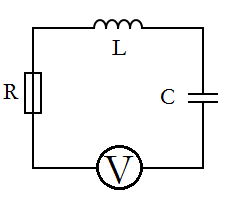
circuitwithnumbers1(Figure 1)

The differential equation that governs this RLC circuit is given by

LI''(t)+RI'(t)+\frac{1}{C}I(t)= E_{0} \omega cos(\omega t) [1]

where L is the inductance, R is the resistance, C is the capacitance, I is the current, \omega is the resonant angular frequency,  E_{0} is an initial value dependent on the voltage source, and t is the time. The inductance (L), resistance (R), and capacitance (C)are all determined by their respective circuit components, which are easily changed out for different ones. \omega depends on the inductance and capacitance, and its value is given by

\omega =\frac{1}{\sqrt{LC}} [2]

What we have left in terms of variables are current (I) and time (t). For our purposes, time is the independent variable, which leaves the current in the circuit at any time to be the dependent variable. Now that we have established this, we can solve our differential equation [1] for current as a function of time (I(t)).

In order to solve [1], I will use the equation solving powers of Mathematica. In particular, the DSolve function is used.  When plugged into Mathematica, the input line looks like:

\text{DSolve}\left[\frac{\text{Current}(t)}{\text{Capacitance}}+\text{Inductance} \text{Current}''(t)+\text{Resistance} \text{Current}'(t)=E_{0} \omega \cos (\omega t),\text{Current}(t),t\right] [3]

We must set values for resistance, inductance, capacitance, and  E_{0}. For this run through of the solution I chose the following arbitrary values:

  • Inductance= 1 Henry
  • Resistance= 10 ohms
  • Capacitance= .1 farads
  •  E_{0}= 1 Volt

When the command is run with the above values set, Mathematica generates the general solution, which is:

I(t)=c_1 e^{-8.87298 t}+c_2 e^{-1.12702 t}+0.040824(-Cos(3.162t)+e^{6.661*10^-16t}Cos(3.162t)-0.3564Sin(3.162t)+2.806e^{6.661*10^-16t}Sin(3.162t)) [4]

First, lets make sure that this solution is reasonable. The known form of the solution to the equation for such a circuit is given by:

I(t)=c_1 e^{r_{1}t}+c_2 e^{r_{2}t}+Asin(\omega t-\varphi ) [5]

The form of our equation [4] seems to match up pretty nicely with this known solution [5]. Now, lets examine [4] in more detail.

Our solution [4] looks a little daunting, but we can break it down into its components. The first two terms have constants that depend on the initial current running through the system, i.e. when I(t)=I(0). However, we can approximate the equation by only looking at the last term, which is a superposition of sin and cosine functions along with a couple exponential terms thrown in. The reason that we can apply this approximation is that the first two terms “damp out” quickly, and thus have exponentially less of an effect as time progresses. The reader may still be curious to see how much of an effect these terms have on the current flowing through the system: to that I say don’t worry! After my initial approximation, I will solve for these constants and compare the two cases.

For now, we will deal with the approximate solution, which is:

I(t)=0.040824(-Cos(3.162t)+e^{6.661*10^-16t}Cos(3.162t)-0.3564Sin(3.162t)+2.806e^{6.661*10^-16t}Sin(3.162t)) [6]

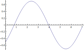
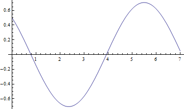
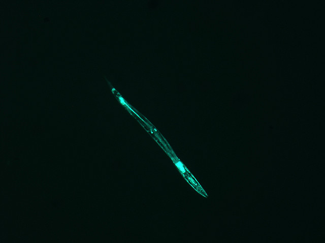
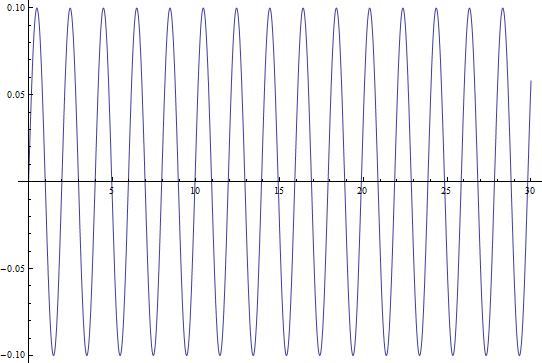
Now that we have this equation, we can use Mathematica to give us an idea of what the changing current looks like over a longer period of time. Figure 2 shows the current in the circuit as a function of time (I(t)) plotted over a 30-second interval.

30secondplot(Figure 2)

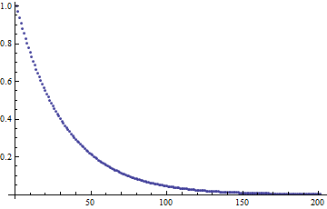
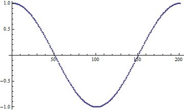
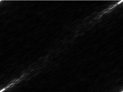
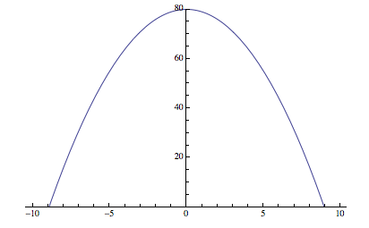
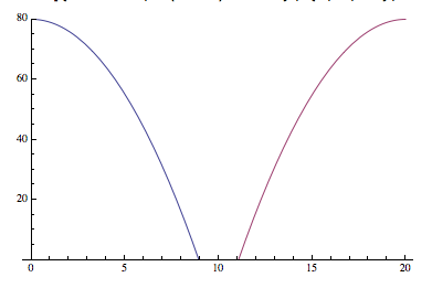
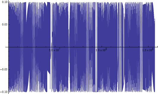
This looks like something we would expect! A sinusoidal wave that describes the changing current over time, just like our equations dictate. But, this is a short time-scale. What happens when we look at the changing current over a longer period of time? In Figure 3, I show the changing current over a longer time period (3000 seconds/50 minutes). In Figure 4, I repeat the process, but with the timescale being 5 years.
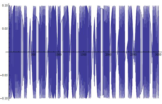
50minuteplot(Figure 3)

5yearplot(Figure 4)

In both Figures 3 and 4, we see some very interesting long-term variations in the current. Why does this occur? Well to be honest, I am not completely certain. I do have a few ideas though:

  • My first inclination is that the long-term variations are in part due to the approximation I made by removing the first two terms of Equation [4].
  • My second idea is that these long-term structures are present due to a possible approximation Mathematica may have made when solving the differential equation.
  • My third and last thought is that these variations are not an artifact of finding the solution, but truly do exist in this theoretical circuit I have chosen.

Why?

A question that the reader may have after looking at all of this is “Why is the long-term structure important?” The answer lies in the fact that RLC circuits are embedded in many electronic devices, including radios and televisions. For this reason, it is important to know the current they put out. We don’t  really want something that has an unpredictable output in devices that are high-cost.

Forward Plan

To further investigate the reason for the long-term structure, I will first solve for the constants in Equation [4] and plot the graphs of current again. Hopefully this will provide some insight into the workings of the circuit. I may also alter the initial parameters (inductance, resistance, etc.) to see if this provides any insight. If not, then I will investigate Mathematica’s differential equation solving techniques and attempt to alter my solution in a way that provides a more accurate solution.

Resources

1. Circuit Diagram Maker- http://www.circuit-diagram.org/

2. The RLC Circuit- University of British Columbia-  http://www.math.ubc.ca/~feldman/m121/RLC.pdf

3. Mathematica Cookbook by Sal Mangano

Mathematica Notebook

https://drive.google.com/file/d/0B3mtB6CQNnpjejEzN25zbFlqajQ/edit?usp=sharing

Share

Relativistic E&M: Preliminary Results

It is fairly easy to see that the electric and magnetic fields of various systems change drastically when considered in different reference frames. For example, consider a wire with a line of positive charges moving to the right at speed v, and an equal line of charges moving to the left at speed v.

current wire B only

This system has a net charge of zero, so there should be no electric field. However, the sum of the charges does cause a total current I = 2λv to the right, which gives a magnetic field of B = μ0λv/πs in the ϕ direction (as dictated by the right-hand rule), for any distance s from the center of the wire.

current wire B0 vector

Now, consider the same situation, but in the reference frame where q is at rest. Suddenly, the positive linear charge is much smaller than the negative one, leaving a net negative charge on the wire, which will produce an electric field. Simply by changing the reference frame, the situation switched from a purely magnetic phenomenon to a combination of electric and magnetic.

current wire EB

However, rather than trying to analyze the magnitude of the new charge and current values to find E and B, it is possible to simply use the following transformation equations to find out what the new E and B fields are.

$E’_x$ = $E_x$
$E’_y$ = $\gamma$ ($E_y$ – $vB_z$)
$E’_z$ = $\gamma$ ($E_z$ – $vB_y$)
$B’_x$ = $B_x$
$B’_y$ = $\gamma$ ($B_y$ + $\frac{v}{c^2}$ $E_z$)
$B’_z$ = $\gamma$ ($B_z$ – $\frac{v}{c^2}$ $E_y$)

Where $\gamma$ = $\frac{1}{\sqrt{1-{\frac{v^2}{c^2}}}}}$ (From Griffiths Introduction to Electrodynamics, 3rd Ed. p531). The only hiccup is that the original setup is in cylindrical coordinates, while the transformation equations are in Cartesian. However, Mathematica can do this automatically, so I’m going to leave it in these terms.

B-field:current wire B1 vector E-field:current wire E1 vector

The Mathematica file contains 3D vector plots of the E and B fields for the rest frame and a frame moving at v=0.25c, but so far, I haven’t figured out how to make it so that the user can vary the speed of the reference frame. Hopefully, I will figure that out soon. The key thing to note is that the model shows the interplay of E and B fields at relativistic speeds: the scenario starts out completely magnetic and ends up a mix of the two.

Share

Preliminary Results: Modeling E and B Fields of a Toroidal Conductor to Explore Tokamak Plasmas

Thus far, I have determined values for the quantities of interest (except for $\mu$ of the plasma) and I have derived an expression for and H.  I will base the parameters of my model off of the Joint European Torus (as per Albanese, et al., 03; Crisanti, et al., 03). It appears that there will be no field, since the plasma is a conductor and would not polarize, but simply experience a current.

  • $q(r) = \frac{r B_{\phi}(r)}{R B_{\theta}(r)} = 3$
  • $r = .95~m$
  • $R = 2.85~m$
  • $I = 6.0~MA$

I am going to assume that N, the total number of turns, is proportional to the safety factor: $N = \alpha q(r)$ where $\alpha$ will probably be related to the circumference of the torus (which can be found from the radii).

The Biot-Savart Law gives:

$d\textbf{B} = \frac{\mu_{0} \textbf{I} \times \textbf{r} dl}{4 \pi r^{3}}$.

If we assume that the torus is in the x-y plane, centered at the origin, and consider a test point at $\textbf{r}$ and source charge elements at various $\textbf{r’}$.  Then $\scriptr = \textbf{r} – \textbf{r’}$.  Consider a test point on the x-z plane.

Assuming that the winding is tight enough, we can say that $ \textbf{I} = I_{s} \hat{s} + I_{z} \hat{z}$ which, in cylindrical coordinates, is $(I_{s}cos(\phi), I_{s}sin(\phi), I_{z})$.

In evaluating the Biot-Savart Law, we have the term $\textbf{I} \times \textbf{r}$.  Due to the symmetry of the tours, the x and z components cancel out, leaving just a y component.  If the test point is in the x-z plane, this means that the magnetic field will be circumferential, or in the positive $\hat{\phi}$ direction.  The magnetic field can then easily be found using Ampere’s Law:

$\textbf{B(r)} = \frac{\mu_{0} N I}{2 \pi s} \hat{\phi}$

for all points within the minor radius (inside the torus) and

$\textbf{B(r)} = 0$

for all points outside the torus.

From here, it is also easy to find the Auxiliary field, from $\textbf{H} = (1/\mu) \textbf{B}$, so

$\textbf{H} = \frac{1}{\mu} \frac{\mu_{0} N I}{2 \pi s} \hat{\phi}$

inside the torus and

$\textbf{H} = 0$

outside the torus, since there is no magnetic field.

I have also begun work on my Mathematica model.  I began by trying to figure out how to get the vector field to look right, and have been working with a simplified version of my equation, $\textbf{B} = k/r$.  I have found that the transform to spherical coordinates is easiest to work with (since toroidal geometries do not fit easily into either spherical or cylindrical), which is why my expression uses r instead of s.  This has given the following vector field:

The (simplified) circumferential magnetic field due to a toroidal solenoid (without taking into account the fact that the field is zero outside of the loop of the solenoid).

The (simplified) circumferential magnetic field due to a toroidal solenoid (without taking into account the fact that the field is zero outside of the loop of the solenoid).

The vector field is the shape that I need it to be, but I’m having some trouble getting the field to be zero outside of the solenoid.  I tried to use the piecewise function of Mathematica, but keep getting an error.  I think I may need to define two fields (maybe 3) such that they cancel out in the regions where the field should be zero.

The next step will be to input the numbers into my expression, and work out the Mathematica model.  Then I will be able to easily vary q(r) and observe the results.

Link to Mathematica notebook: https://drive.google.com/file/d/0B-C9MvBAfmyIQS12dTZJOGh5bm8/edit?usp=sharing

References

Raffaele Albanese, G Calabr`o, M Mattei, and F Villone. Plasma response models
for current, shape and position control in jet. Fusion engineering and design,
66:715–718, 2003.

F Crisanti, R Albanese, G Ambrosino, M Ariola, J Lister, M Mattei, F Milani,
A Pironti, F Sartori, and F Villone. Upgrade of the present jet shape and vertical
stability controller. Fusion engineering and design, 66:803–807, 2003.

Griffiths, D. J., & Reed College. (1999). Introduction to electrodynamics (Vol. 3). Upper Saddle River, NJ: prentice Hall.

Share

Preliminary Data

Using Gauss’s Law for the Electric Field, I found the electric field for a conducting cylinder with a charge density

CodeCogsEqn .                                                               (Eq.1)

The end result is the equation

.                                                          (Eq.2)

With this, I was able to model the following.

Efield for conductors                                           (Figure 1)

Here is a photo of what is occurring on the inside of the cylinder. As you can see in Figure 2, the Gaussian surface would be placed in the center of the cylinder where the vector fields start and are directed radially outward.  As implied by Equation 2, the electric field is directly proportional to the radius of the cylinder.

efield inside                                            (Figure 2)

I am currently working on modeling the magnetic field.


Share

Preliminary Results: C. elegans Diffraction Pattern Modeling

Staying true (so far) to my tentative project timeline, I acquired images of the C. elegans in various shapes, I have done quite a bit of research on Fourier Transforms and Fraunhofer Diffraction, and so far I have successfully transformed one image into the corresponding diffraction pattern.


IMAGE 1

sampleworm1I took this image and used Screen Shot 2014-04-21 at 5.16.08 PMmathematica to sharpen it –> setting it to grayscale and brighten it –> collect dimensional information –> apply a Fourier Transform, yielding (after some similar image manipulation):

This is a great diffraction pattern, but I had issues with the poor resolution and general image quality. To remedy this, I proceeded with images taken with a higher-resolution camera.

(full file for image 1: book 1 )

IMAGE 2

3975815904_e33a49b65b_z

This beautiful image needed some manipulation, similar to image 1: I converted it to grayscale –> brightened it significantly (to make it a more definite shape, and to get rid of the “holes” in the luminescing nematode)  –> collected image dimensions and data –> applied the FT. Unfortunately, I ran into a problem.

The produced image:

Screen Shot 2014-04-21 at 5.31.56 PM

Obviously this is quite different than the first diffraction image.

I had a few hypotheses:

1. The image was saved as a .jpg, but the same image was produced when I tried again with a .png version of the image.

2. The computer is phase- shifting the image so that instead of the origin lying in the center of the product, it is splitting the right side from the left side and lining them up in the wrong order. How can I rearrange and correct the phase shift in the output?

An analogy to the second hypothesis:

Screen Shot 2014-04-21 at 5.45.39 PM

Screen Shot 2014-04-21 at 5.45.53 PM


—>


It is as if, instead of centering the origin in the center of the produced diffraction pattern, the computer is putting the “origin” in a different place, and splitting the image, similar to the parabola I produced above.

My solution is a little underhanded. I divided the image into four equal rectangles, and manually rearranged them to produce what I knew was the true image:Screen Shot 2014-04-22 at 7.52.00 PM

(full file for image 2: book 2a  book 2b )

—————-

Reflection:

It is important to keep this process grounded: how is this relevant to Electromagnetism? The answer is that this entire process is only viable because of the laws of electromagnetism. I am analyzing the images by taking their Fourier Transforms. The diffraction pattern is the FT of the function that describes the electric field strength across the aperture of diffraction. In other words, I am applying an operation (the FT) to the image, which is a direct indication of the electric field strength across the aperture (the microscope slide) to mathematically find the diffraction pattern produced by the specific electric field array created by the shape of the worm.

Specifically, the diffraction pattern here is the Fraunhofer Diffraction pattern, or “far-field” diffraction, which occurs when the distances between the screen, aperture, and light source are appropriately far $L>>\frac{b^{2}}{\lambda}$. Diffraction effects are an outcome of the type of light wave.

It is also essential to realize what information is lost in the computation of these diffraction patterns. I am taking a real image, applying a FT to it, squaring the absolute value of the result, and arriving in a complex space. This process loses the phase information of the light, and as a result, it is possible to go from the image to the diffraction pattern, but impossible to find the image from the FT diffraction image.

Share

Project Plan

In response to Professor Magnes’ primary question, whether I will be modelling the E/B fields or the forces acting on moving bodies, I intend to do both; in particular I have the opportunity to illustrate the Lorentz covariance if I show the forces acting on the magnet and conductor. As covariance is a bit more challenging a concept than invariance I think this illustration and discussion will be a good teaching tool.

I am also trying to find a way to illustrate the changes in the electromagnetic field one would observe as they moved relative to various objects. Mathematica’s animate command should be aptly suited for this as I could use the t-parameter as a scalable velocity term.

My first and most important goal will be to do a brief write up of the EM inspiration for relativity and accompany this discussion with an illustration of Einstein’s magnet and conductor thought experiment. I intend to have these completed by this upcoming Friday (4/18).


I will spend my weekend looking for the more interesting examples of field transformations I can incorporate into my project and intend to have them animated in my preliminary upload on Tuesday.


I have also come up with a few arbitrarily designed plots of the affect of length contraction on observed charge density which I also intend to have polished up a little bit and incorporated into my preliminary upload as well.

Share

Revised Project Plan: Relativistic E&M

So it seems that step 1 of my original plan is more involved than I thought. To satisfactorily derive the E- and B-field transformation equations, it would be necessary to delve into the depths of relativistic mechanics, including the transformation of equations for motion, momentum, and energy, among others. This seems like it is outside the scope of the project: indeed, Griffiths spends about 55 pages before he is able to state the field transformation equations. I thought there would be a point halfway through at which I could pick up and start the derivation, but I was incorrect, so I am going to take the transformation equations as given, and work from there.

That being said, my new timeline will be essentially the same as the old one, just starting at what used to be Step 2 with the application of the transformation equations to one or two situations.

1) 4/14-4/18: Pick one or two simple scenarios and find their E- and B- fields if they were traveling in a moving reference frame. This will be a computational step. The transformation equations are pretty straightforward, so it should take less time. This is just to have a proof of concept, so it is less important that the system has interesting behavior in a moving reference frame.

2) 4/18-4/24: Make 3D or 2D vector field models of these situations in Mathematica. This portion will be focused on figuring out how to make mathematica do what I want. The goal is to come up with an animation or interactive figure that can be used to view the vector fields when the system is moving at different speeds, starting at non-relativistic speeds and working up to the speed of light.

3) 4/24-5/2: Find and model situations that display either representative or unusual behavior when considered in a relativistic reference frame. Once the Mathematica simulation for the first situation has been figured out, the following cases should be easier to take care of. Interesting behavior might include systems that only have an electric field in one reference frame and only a magnetic frame in another. It also may be interesting to consider what happens if a reference frame is moving faster than the speed of light.

4) 5/15/14: Summarize results and write conclusions. This will consist of a final look at the systems considered earlier and suggest possible directions for future exploration.

Share