Group 5 Project Data

The majority of our project was done mathematically, using data collected from NASA’s logs of asteroids that came within sensor range.

The collision of any asteroid with Earth could prove catastrophic:

NEO diameter (m) larger than:
Average interval between impacts (years)
Energy released (megatons of TNT)
Crater diameter (km)
Possible effects/comparable event
0.015 Hiroshima atomic bomb detonation.
30 300 2 Fireball, shock-wave, minor damage.
50 2000 10 ≤1 Tunguska-type explosion or small crater.
100 10,000 80 2 Largest H-bomb detonation.
200 40,000 600 4 Destruction on national scale.
500 200,000 10,000 10 Destruction on continental scale.
1000 600,000 80,000 20 Many millions dead, global effects.
5000 20 million 10 million 100 Billions dead, global climate change.
10,000 100 million 80 million 200 Extinction of human civilization.

(Table from Alan W. Harris (US) “Estimating the NEO population and impact risk: past, present and future” presented at the 1st IAA Planetary Defense Conference, 2009)

As previously mentioned, the NEOShield Project has put forth three possible solutions would handle an asteroid on a direct collision course to our planet; the kinetic impactor, nuclear blast deflection, and gravity tractors. In order to mathematically simulate the outcome of these countermeasures, we first generated two asteroids (A and B) to satisfy both extremes and allow us eventually interpolate a trend in the force needed to mitigate their flight;

Given that the average density of an asteroid is 4.95 g per cubic centimeter then:

(1)   \begin{equation*} Masteroid= 4.95 * \frac{4}{3}π^3 \end{equation*}

DIAMETER MASS REL. VELO. DIST. FROM EARTH
Asteroid A 4.1 km 1.79 E14 kg 33,100 m/s 1.89 E10 m
Asteroid B 40 m 1.66 E8 kg 6,500 m/s 1.89 E10 m

Note that the distant is constant. Also, the minimum requirement needed is to delay the asteroid by a period of 420 secs., which is the amount of time it takes Earth to move the distance of one planetary diameter, and the asteroid to pass “safely” by.

Kinetic Impactor: The weight of the Impactor is 650 kg 

Asteroid A: 

(2)   \begin{equation*} Time until Impact = \frac{distance}{velocity} = \frac{1.89E10}{33,100} = 570,997 secs. \end{equation*}

(3)   \begin{equation*} New Velocity = \frac{distance}{new impact time} = \frac{1.89E10}{571,417} = 33,075.67 \frac{m}{s} \end{equation*}

(4)   \begin{equation*} Deceleration = V1 -V2 = 33,100 - 33,075.67 = 24.33 \frac{m}{s^2} \end{equation*}

(5)   \begin{equation*} Force Needed = mass*acceleration = 1.79E14 * 24.33 = 4.36E15  N \end{equation*}

(6)   \begin{equation*} F = mΔv= m(V1-V2) \end{equation*}

(assume V2= 0 for complete inelastic collisions)

(7)   \begin{equation*} 4.36E15 = 650* V1, V1= 6.7E12 \frac{m}{s} \end{equation*}

This is faster than c, and would be improbable ! A kinetic impactor would not be used on an asteroid of this size.

Asteroid B: Using the same equations as above  with the appropriate substitutions, we are left with:

Impact Time with Delay = 2,908,112 secs.

New Velocity = 6,499 meters per second

Deceleration =  1 m/s

Force Needed = 1.66E8

V1 = 255, 385 meters per second.

This is a plausible solution in the friction-less vacuum of space, as the impactor could reach this velocity.

Nuclear Bomb Deflection:

For this mathematical simulation, we assumed that the standard B53 nuclear warhead would be employed, which has a 9 MT yield, giving off approximately 1.25E6 N of force if detonated at 30m from the asteroid.

Asteroid A:

F= ma 

1.25E16 = 1.79E14a

Solve for a = 70 meters per second squared

New Velocity = 33,030 meters per second

Initial Impact Time = 570, 997 secs. , as given by:

(8)   \begin{equation*} t = \frac{d}{r} = \frac{1.89E10}{33,100} \end{equation*}

New Impact Time = 572, 207 secs, given the delay of 1210 secs. (approx. 20 mins.)

This would slow this asteroid down at three times the magnitude needed for Earth to reach a safe position on its orbit.

Asteroid BUsing the same formulas (with the appropriate substitutions as above):

a= 75,301, 204 meters per second squared

New Velocity = 75, 294,705 m/s away from Earth, if not immediately vaporized.

This wouldn’t just slow down Asteroid B, it would send it hurtling in the exact opposite direction. Using such a method on an asteroid of this size would be the definition of overkill!

Gravity Tractor:

This method operates on deploying large “satellites” capable of sustaining and orbit around the asteroid in question and dragging it away from its original vector using gravity over a long period of time.

This operates on the equation:

(9)   \begin{equation*} F = G \frac{Mm}{r^2} \end{equation*}

Where: is the universal gravitational constant, is the mass of the gravity tractor(s), m is the mass of the asteroid and r is the distance the asteroid is from Earth.

Gravity Force

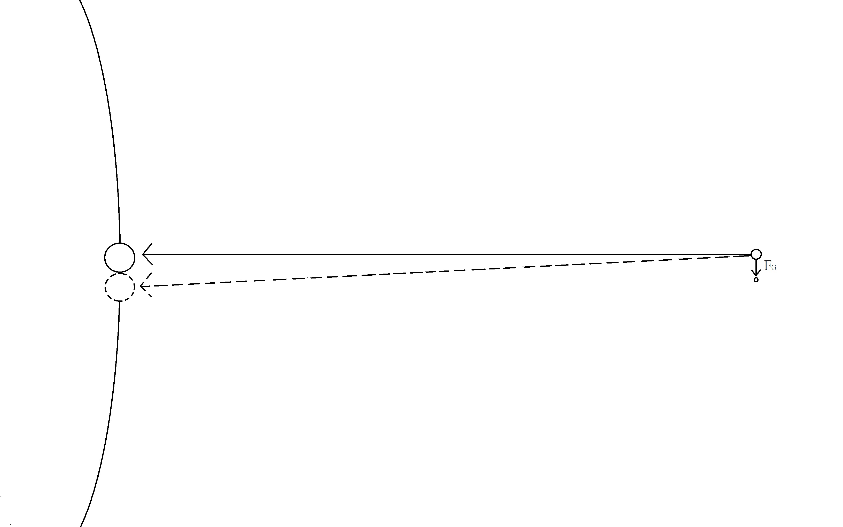
The diagram above depicts the path the asteroid would need to be “nudged” onto in order to safely miss Earth. At the given distance of 1.89E10 meters, it is impossible to calculate how much gravity will affect the asteroid in relation to our planet; there are too many variables, and the angle that the asteroid would need to be deflected is so infinitesimal that the mass of the gravity tractor would be unquantifiable. The gravity tractor could only be used at much greater distances over a span of decades, and even though, as a primary counter-measure to allow for easier mitigation using the kinetic impactor, or in the most serious of events, a nuclear explosion.

Visual representation:

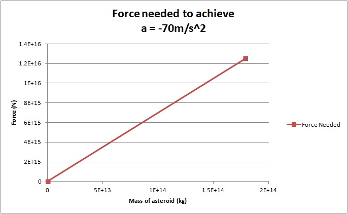
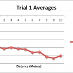
After testing these three methods mathematically, we were able to generate, as promised, a graph depicting the trend of force needed to deflect asteroids of various sizes:

Force graph

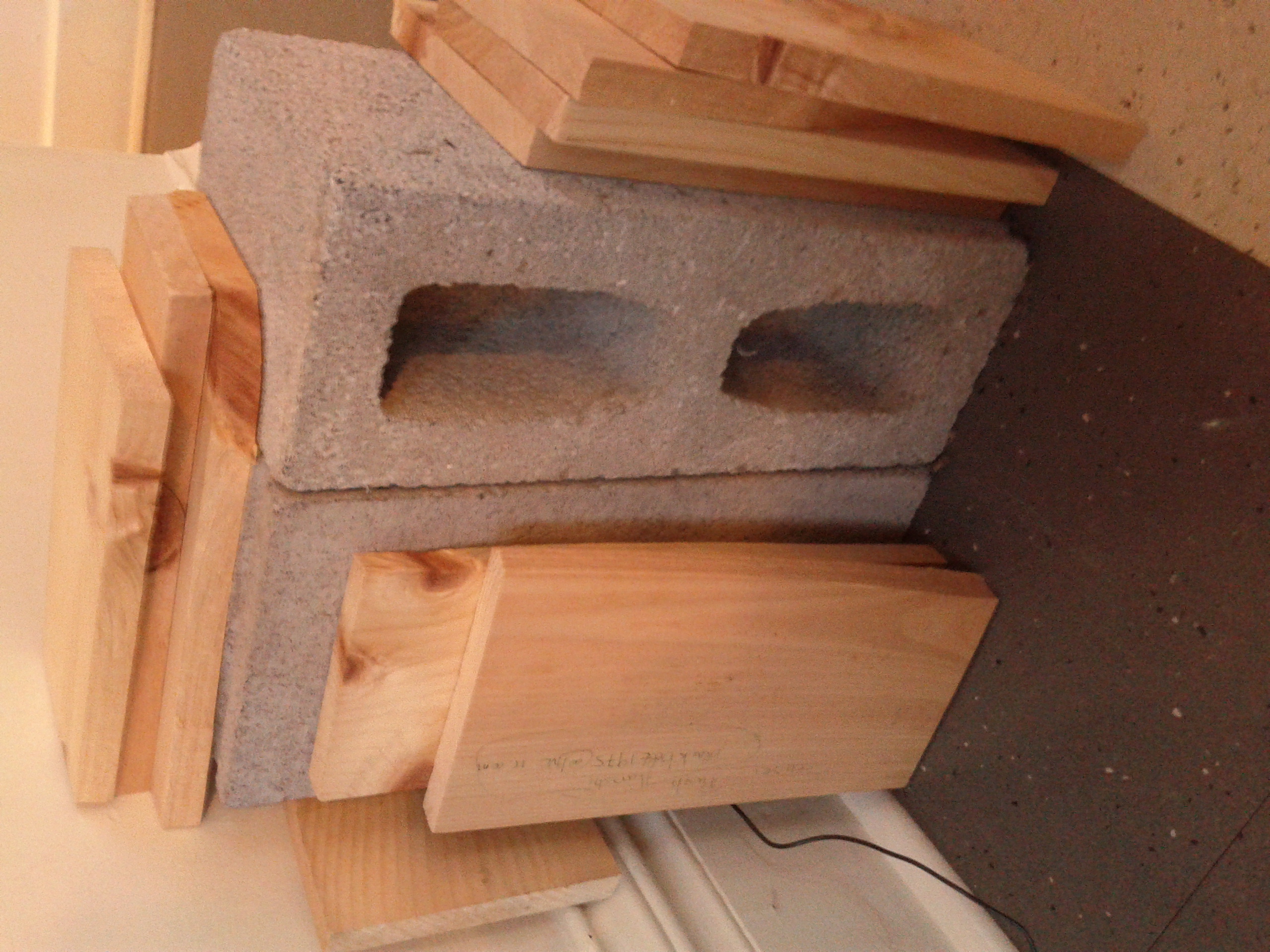
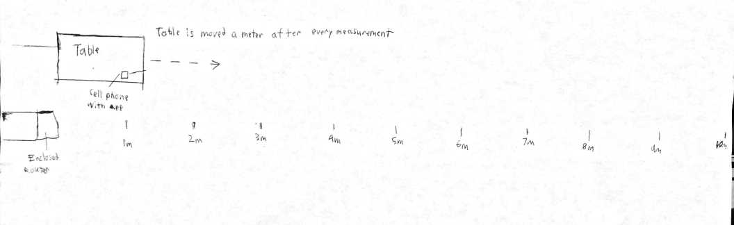
We also filmed a crude recreation of the relative process of  the kinetic impactor: (SOON TO BE UPLOADED), but the process is more expertly (though somewhat overdramatically) represented by the NEOShield PR video.

They also provide a time-table for the employment of the counter-measures.

DSCN3891

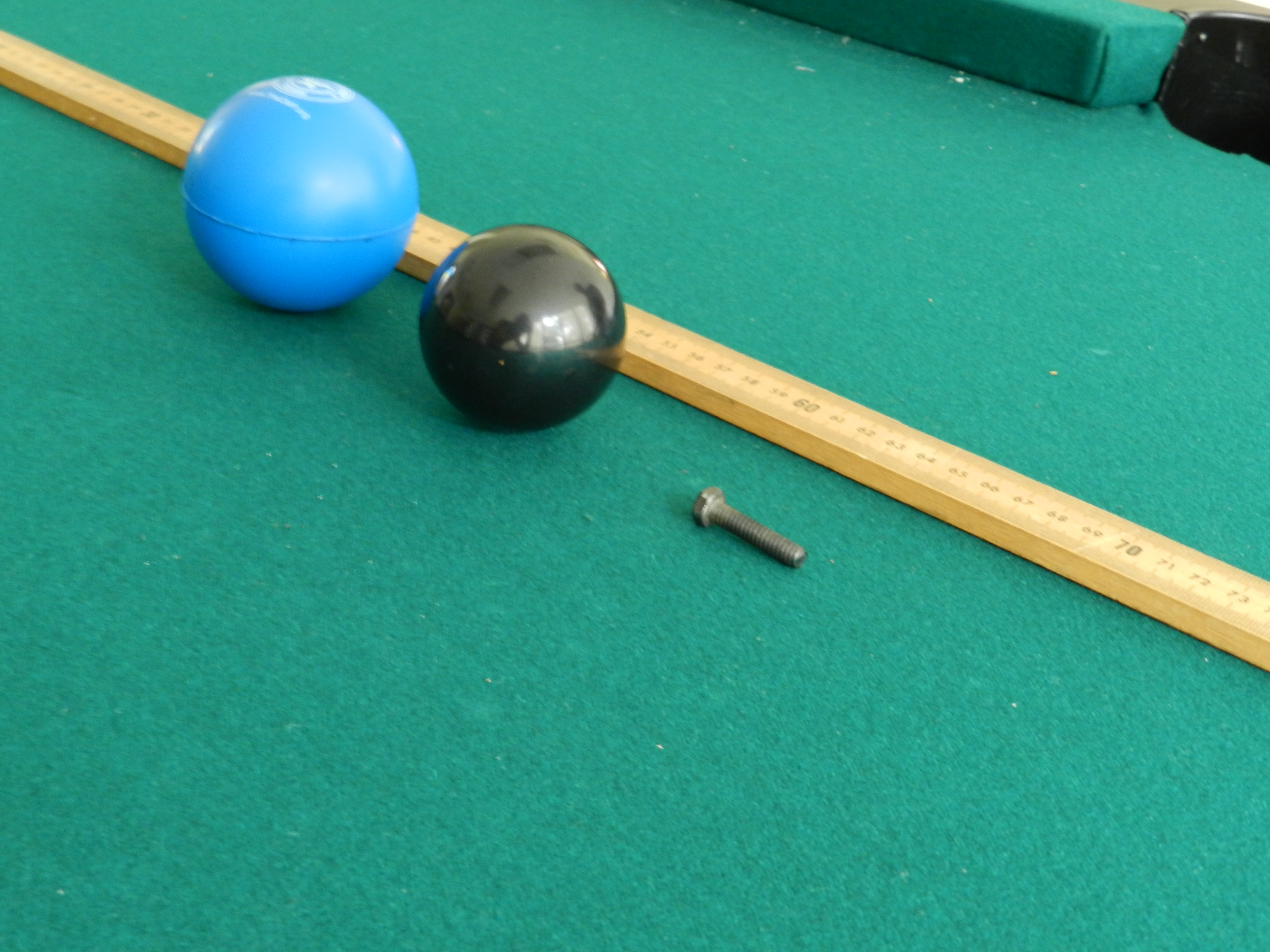
Above: Blue ball (Earth), black ball (asteroid) nail (kinetic impactor), and meter stick (measurement tool). Note that these are not necessarily to scale or proportional to one another, and that as objects moving in space are relative, that the kinetic impactor is represented as static.

DSCN3896 – depicting an uninterrupted collision with Earth

DSCN3898 – depicting the use of a kinetic impactor at nominal range

DSCN3902 – depicting the use of a kinetic impactor at a farther engagement

Data - Bomb 
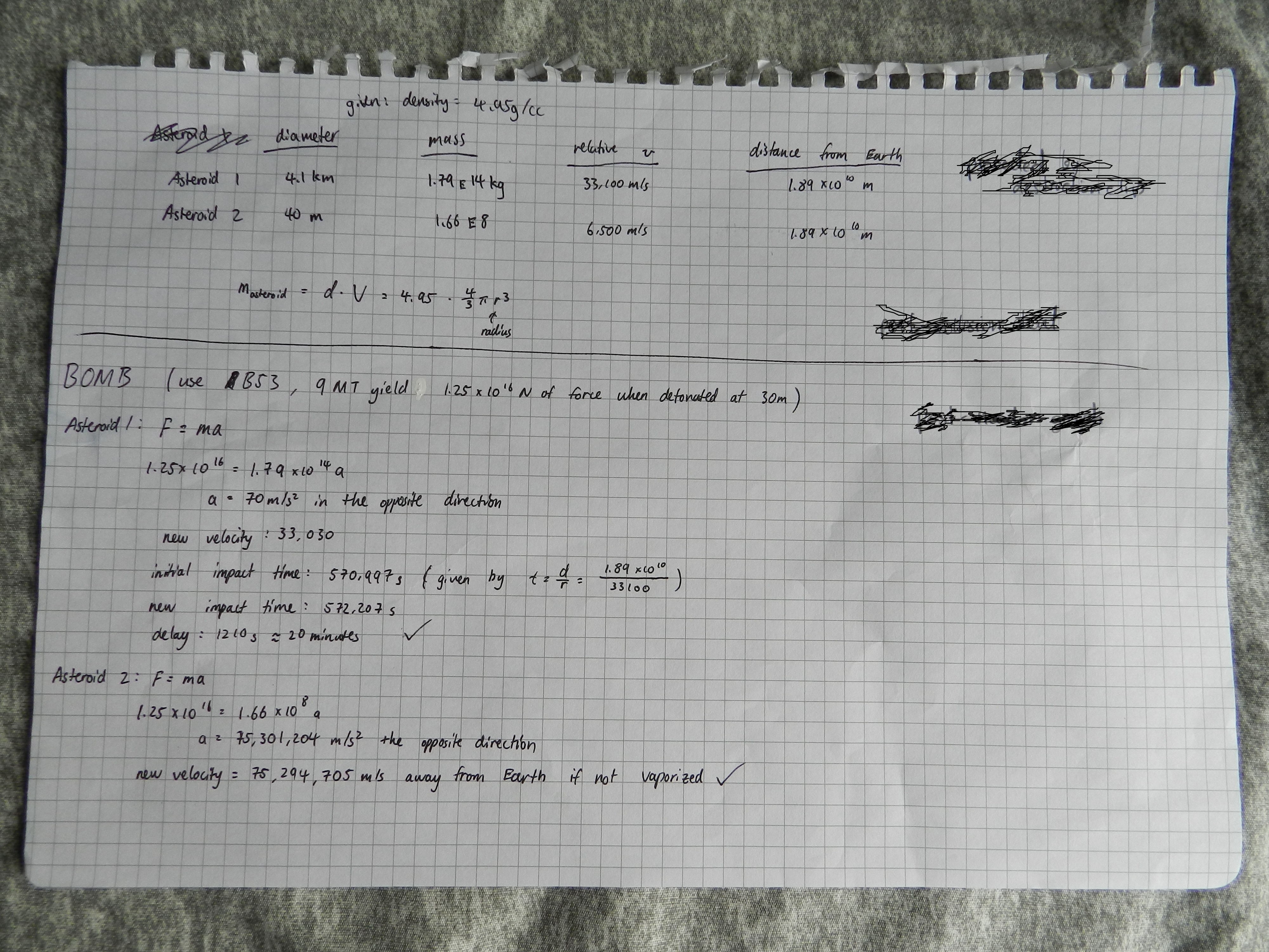
Data for asteroid dimensions and bomb.Data - Kinetic Impactor
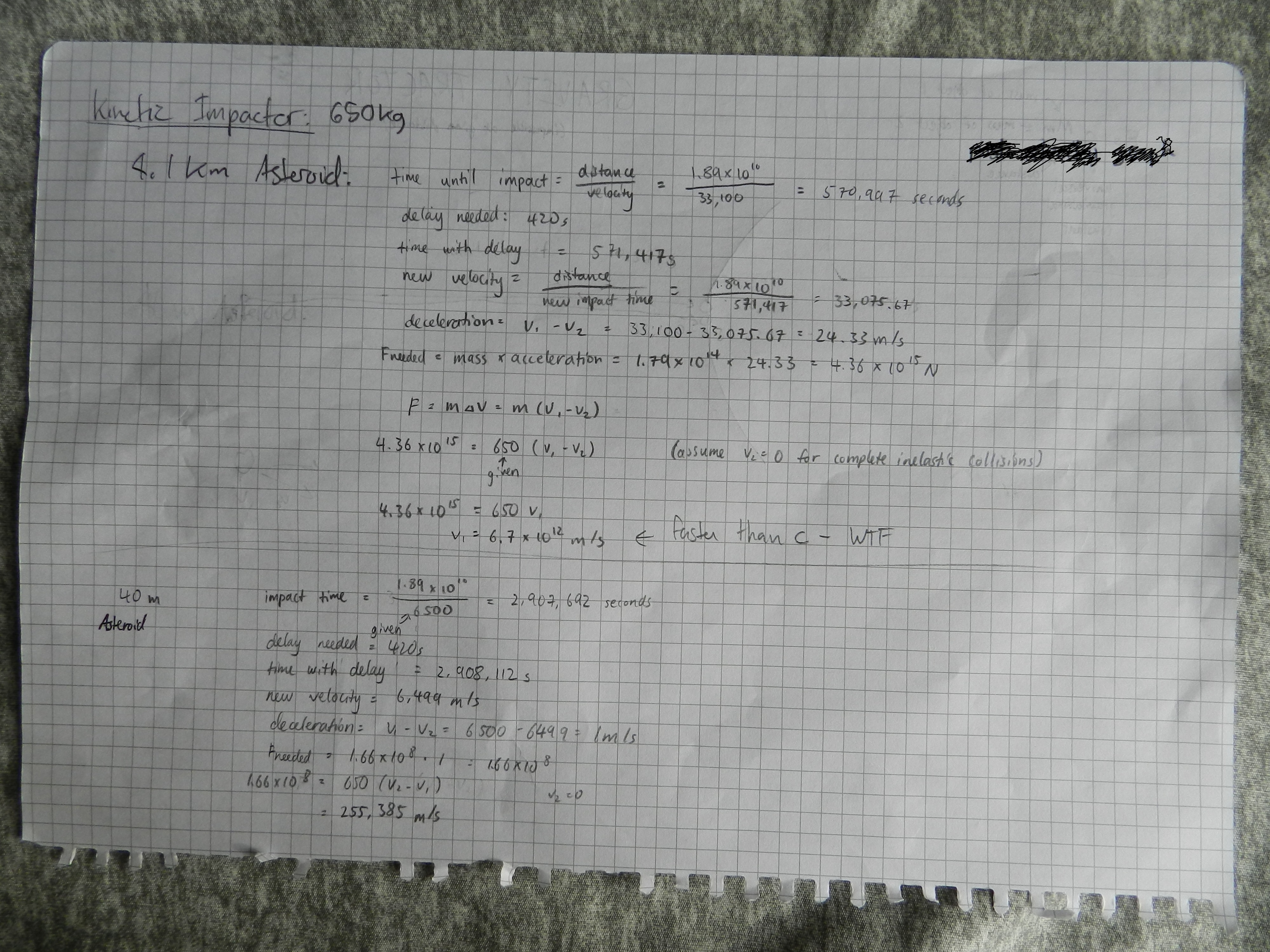
Data for kinetic impactorFormula for Gravitational ForceFormula and theory for gravity tractor.


Group 4 Project Data

Data Collection Methods:

group4trial3

Our router in trial 3, with full enclosure

We set up our experiment in the Raymond MPR, laying out tape in 1m intervals, and placing the router on the floor. We placed the measuring instruments on a table and moved the table 1m back when we had taken enough data at each distance.

Trials 1-3: Using an Android cell phone with the app Wi-Fi Analyzer, we recorded the signal strength of the wireless access point (WAP) from 1-10 meters. The app scans for networks and reports the signal strength, every 5 seconds. Data was taken at 5 second intervals, in which the cell phone app refreshes its readings.

group4diagram

A diagram of our experiment.

Router Conditions for Trials 1-3

In order to modulate our variable, we increased the volume of the medium being passed through by the wireless radio signals during each trial.

Trial 1: WAP uncovered.

Trial 2: WAP covered with cinder block.

Trial 3: WAP covered with cinder block and surrounded by 12 wood planks.

Trial 4: WAP uncovered.

Trial 4: RF Meter used to record mW/m² values. The meter was used on its instantaneous value setting and records values rapidly, so table data was taken in 5 second intervals.

Explanation of Data

In order to make it easier to recognize trends, we took the averages of the 5 data values taken at each distance for trials 1-4 and used those for graphing. We believe that graphing average values is the most logically sound and clear way to represent our data, as the readings for both power density and power tended to fluctuate greatly, making instantaneous values unreliable to graph.

The general trend in our data measurements is that the average power density and power tends to decrease as we increased the amount of obstacles, as we would intuitively guessed. However, it is interesting to note that the trend of the averages in fig 4 has an interesting behavior. At around 9 meters, the readings dip to their lowest values before returning to a higher value at 10m. We suspect that this may relate to the wave reinforcement and/or cancellation— the reflective/absorbent properties of Raymond MPR’s various materials and geometric shape is probably to blame for this peculiar anomaly.

Trial 4 data was not averaged with the other trial data on fig. 4 because the units being compared are not effectively comparable (dBm vs. mW/m²). We found the data for trial 4 to be problematic and unreliable because of the extremeness in fluctuation of the data given by the RF meter. However, the sharp cutoff from 1m to 2m may reveal that radio signals have an unexpectedly steep cutoff. Because of this, smaller increases in distance at this specific cutoff distance (found to be somewhere between 2-3m) may result in great loss of power density. However, this is only a conjecture, as we are wary of giving legitimacy to this data set because the volatile behavior of the RF meter.

Units

mW/m² – Power density (milliwatts per meters squared)

dBm – Power, expressed in a logarithmic ratio (decibel-milliwatt)

m – Distance, standard SI base unit (meters)

Data Tables

Trial 1, without block.            
Distance A B C D E Average
1 -42 -39 -36 -38 -41 -39.2
2 -44 -41 -41 -41 -41 -41.6
3 -42 -38 -41 -41 -38 -40
4 -41 -41 -41 -44 -41 -41.6
5 -41 -41 -41 -47 -41 -42.2
6 -41 -44 -50 -47 -50 -46.4
7 -44 -47 -47 -44 -47 -45.8
8 -53 -50 -47 -50 -59 -51.8
9 -56 -53 -50 -56 -53 -53.6
10 -53 -47 -53 -47 -53 -50.6
Trial 2, with cinder block only            
Distance A B C D E Average
1 -42 -35 -41 -35 -41 -38.8
2 -47 -50 -53 -50 -47 -49.4
3 -48 -41 -44 -50 -41 -44.8
4 -44 -47 -50 -47 -41 -45.8
5 -44 -50 -47 -47 -41 -45.8
6 -48 -47 -44 -50 -50 -47.8
7 -47 -50 -47 -53 -47 -48.8
8 -50 -56 -50 -56 -59 -54.2
9 -59 -53 -56 -59 -53 -56
10 -47 -56 -50 -53 -53 -51.8
             
Trial 3, with cinder block + 12 wood surrounding            
Distance A B C D E Average
1 -41 -35 -35 -41 -35 -37.4
2 -50 -53 -50 -47 -53 -50.6
3 -44 -50 -41 -44 -41 -44
4 -44 -41 -44 -47 -50 -45.2
5 -41 -44 -50 -44 -44 -44.6
6 -53 -44 -50 -47 -53 -49.4
7 -53 -56 -56 -50 -50 -53
8 -56 -53 -56 -56 -53 -54.8
9 -59 -53 -56 -59 -53 -56
10 -57 -54 -51 -60 -51 -54.6
             
Trial 4 RF Meter            
Distance mW/m2         Average
1 1168 1356 1701 1397 2136 1551.6
2 401.3 300.8 345.2 291.4 380.5 343.84
3 211.7 229.6 205.8 190.7 246.6 216.88
4 69.4 105.6 87.4 70 116.4 89.76
5 132.5 88.6 105.4 176.4 235.8 147.74
6 32.4 71.6 43.5 39.2 180.5 73.44
7 44.6 51.1 67.4 57.7 33.8 50.92
8 96.8 328.8 76.3 141.6 274.8 183.66
9 31.1 41.6 89.6 35.7 27.2 45.04
10 59.9 74.9 5.8 131.4 60.2 66.44

Data Graphs/Visualizations

Group 2 Project Plan

Roles:

Brittany and Calais will record the instruments and synthesizers, and help compile data. Jessica will lead in the analysis of the data.


Equipment: Vernier LabQuest 2, Vernier microphone, and Vernier Sound Level Meter (SLM-BTA).

We will primarily be investigating sound waves and the different forms they take on. Using the above equipment, we will record and analyze one tone produced by three instruments (piano, flute, and guitar). Later, we will record the same tones produced by several different synthesizers. We will analyze the data and look for distinctions in the waveforms.

For data collection we must ensure these remain constant throughout:
Same speaker system
Same room, preferably noise cancelling (a practice room in Skinner or a lab)
Same microphone/other equipment


Meeting dates and times:

Sunday Sept. 22nd  –Research synthesizers in the library

Monday Sept. 23 at 11:00 am –Record wavelengths of piano, flute, and guitar

Weekend of Sept. 28th -29th–Record synthesizer’s “piano, flute and guitar”

Sunday Sept. 29th–Compile and analyze data


Expected Outcomes:

We expect to see distinct differences in the waveforms produced by the acoustic instruments versus the synthesizers. While we predict more organic sine waves for the actual instruments, we expect to see the waves produced by the synthesizers take on square, sawtooth, or other waveforms. We will analyze these differences not only visually, but by using equations to approximate each unique waveform and mathematically compare their differences.

Group 1: Project Plan

Motivation:
The innovation of wireless technology has given us convenience in the form of mobility, speed, and efficiency. In addition it has enabled us to go outside our reach to form and keep connections made with people all around the world.

Problem Statement:
There is still a rather inconvenient and significant tether that keeps us from moving with the speed and flexibility that we are capable of, the need for electrical power to be transmitted through wire. The solution: Wireless Power Transmission (WPT).

Approach:
There are a handful of products, known as power mats, on the market that offer WPT for the use of charging cell phones and iPods. The purpose of our investigation is to collect data and analyze the commercial products and with that information build a WPT device of our own. Moreover, we wish to consider the limits, benefits, and further applications of such technology.

Results:
Our device will work by inducing a current with a changing magnetic field. By running current through a primary wire, a magnetic field is created, a secondary receiver coil will experience a change of magnetic flux and thus cause current to run through that coil.

Equipment:

  • Watts Up Pro to measure the needed power to run the power mat as well as to measure the power that is transmitted to the receiver coil in the external device.
  • Magnetic Field Sensor to measure the magnetic field around the coils.
  • Temperature Sensor to measure how the primary and secondary coils heat over time and with different power settings.

Roles:
Juan and Elijah will split up the work on collecting and analyzing data as well as the building of the device evenly. Juan will take care of most of the posts on this website.

Activity Plan:
9/23 – Use Watts Up Pro to measure electrical power and the magnetic field sensor for the magnetic fields present
9/24 – Analyze the data from the measurements
9/25 – Read research papers from Scopus covering WPT
9/26 & 27 – Prepare a plan for building the device and order needed materials
10/2 – Post data onto moodle
9/30-10/4 – Build the WPT device
10/5-8 – Collect data on our device
10/9 – Post data and project results onto moodle

Group 5 Work Plan

Equipment List:
x 1 High speed camera
x 1 Meter stick
x 1 Large metal ball
x 1 Small metal ball
x 1 Computer

Set-up of demonstration:

The basic idea is to have a bird’s eye view of the test model within a circular area with a specific radius where the smaller ball (the kinetic impactor) would be launched from a central launching point (assumed to be Earth) at a larger ball (the asteroid) to collide and deviate the larger ball off-course. There will be different speeds of the smaller ball to determine the optimal parameters necessary to deflect an asteroid coming towards Earth without catastrophic effects.

Week of September 23rd:

Monday

Diagram model for camera set-up.

Wednesday

Start filming deflector (kinetic impactor) model. Measure input data (how heavy are the objects and distance).

Friday

Continue filming. Extrapolate data from model to generate an asteroid of randomly generated dimensions for mathematical models.

Week of September 30

Monday

Model gravity and nuclear blast impact through mathematical equations.

Tuesday

Enter LaTex + data

Wednesday

Post.

Week of October 7

Monday

Write conclusion and compile results.

Tuesday

Post.

Group 4 – Wi-Fi Penetration through a Medium – Project Plan

Roles:

Charlie – Collect/manage data, location scouting, manage materials, research information

Richard – Collect/manage data, presentation editing work, file management, research information

Equipment/Supplies:

  • TES-593 electrosmog meter

  • Cell phone (with application for displaying dBm reading)

  • Wood blocks

  • Router

  • Laptop computers (used for documentation and data organization/presentation)


Science/Technology involved:

We will be examining the nature of a specific wireless communication technology known as Wi-Fi. Wi-Fi is a technology used in every almost personal device that accesses the Internet. It uses radio technologies called 802.11, and occupies specific bands of the radio spectrum: 2.4gHz and 5gHz. (Reference)

Radio power levels are measured in decibels (dB), which Cisco Systems defines as “the power of a signal as a function of its ratio to another standardized value.” Our consumer devices often give a reading of the signal strength as (dBm), which is a value compared with milliwatts. (Reference)

Activity Plan

We will be utilizing a TES-593 electrosmog meter. The meter is capable of measuring radio frequency (mV/m,V/m), magnetic fields (µA/m, mA/m), and power density (µW/m², mW/m², W/m², µW/cm², or mW/cm²). The frequency range for the ElectroSmog Meter is 10MHz to 8GHz. With the electrosmog meter, we will be measuring power field density.

To measure electrical power, we will be using a cell phone or laptop, which will provide readings in dBm

First, we will find a location where there is minimal outside interference.

Before we record our data, we will take a control value that accounts for ambient RF activity, since there will most likely be some sort of RF activity present in any locations on campus, due to the high concentrations of RF-emitting devices on campus (wireless networks, cell phones, radio towers, etc…).

When a test location is found, we can set up our experiment.

The router will be placed on one side of the room and powered on to broadcast a network that we will be connecting to in order to gauge its strength.

On the opposite side of the room, we will set up our receiving/measuring devices, which we will use to record data. Our laptops and our cell phones will be used along with a program that will allow us to measure the dBm readings. We will increase the volume of the wood blocks in front of the router and in front of the device, and record the changes in data.

Project Dates:

9/23, 2-4PM; 9/26, 4-6PM; 9/27, 5-7PM; 10/1, 4-6PM

Outcomes:

We believe the general trend will be a decrease in power field density (mW/m2) and a decrease in power level (dBm) that is related to an increase in the volume of the wood— a variable we will be altering and observing.

Group 3 Project Plan


Roles:

Each member of the group will collect the same amount of data. We will each analyze 7 Apple Brand laptops. The laptops we examine will be MacBooks, MacBook Pros and MacBook Airs from 2008 onward. We will then all work together to analyze the collected data through the use of graphs. From our analysis we will collectively write a conclusion explaining our results.


List of Equipment and Supplies:

  • WattsUp? Pro (3)

  • Apple Laptops (21)


Science and Technology:

Through the use of the WattsUp? Pro, we will determine the the power usage of different laptops using different brightness configurations. Since power=energy/time, we will determine how much energy the laptops use of a period of one hour by using the WattsUp? Pro’s energy measuring capabilities. This information is extremely applicable to daily life because it can be used to calculate how much it will cost to run a laptop on different brightness levels, as well as how rapidly the laptop’s battery will be exhausted based on its brightness. This can help users decide how much battery they can actually save by lowering brightness and adjust the brightness levels to their needs.


Activity Plan:

The first part of our project will be to collect the data about the laptops’ screen brightness. Each member of the group will collect the same amount of data using the WattsUp? Pro. We will each record the power usage of Apple Laptops, including MacBook Pros and Airs of different models, at approximately 25%, 50%, 75%, and 100% brightness and then combine our data into one aggregate. We will collect our data during the week of 9/23-9/28, and then meet the following week (9/30-10/5) to combine and analyze our data. We will finalize our project and draw conclusions from our analysis during the week of 10/7.


Expected Outcomes:

We expect that lowering the brightness of the screen will significantly decrease the battery consumption on every laptop that we test. We anticipate that lowering the brightness will decrease battery consumption at a consistent ratio.


Exploring Near Field Communications

Abstract

“Near Field Communication” (NFC) is a set of wireless standards designed to establish communication between devices at a range of 0-5cm. NFC-enabled chips, known as tags, do not require batteries and are instead powered by induction of magnetic fields. When the magnetic field of one device passes close to another, the contactless energy transfer allows small amounts of data to be transferred between the tags. NFC chips are most frequently included in smartphones, enabling a plethora of use cases. Prominent utilizations include NFC-enabled boarding passes, event tickets, contact information sharing, and social media (i.e. tweeting, Foursquare checkins).

One significant limitation of NFC is its inability to function in close proximity to a metallic surface or other ground plane, which disrupts the magnetic signal. We will attempt to counteract this disruption by using different permeable materials to separate the NFC tag from a metallic surface. We hope to amplify or intensify the magnetic field utilized by NFC devices and potentially increase the range at which data transfers are possible by testing different casings and structures of permeable metals.

Materials

NFC tags of varied sizes, embedded in stickers
Thin metal sheeting (iron, steel, electrical steel, permalloy, cobalt-iron, mu-metal)

Schedule

9/19 – Inquire about materials from physics department
9/23 – Trip to the hardware store to find materials / testing
9/25 – Testing / data collection
9/30 – Testing / data collection
10/2 – Final data collection, collect and summarize results
10/7 – Write conclusion
10/9 – Any leftover work

Methodology

An average range of transfers between NFC tags without any metal backing will be established. Inoperability of data transfers when on a metallic surface will be tested and verified. Permeable materials to separate the NFC tag from a metal backing will then be introduced one at a time, and the average range of successful transfers will be recorded. Next, attempts to amplify or direct unadulterated (normal) transmissions with a housing or casing of highly permeable material will be made; the effectiveness of such housing, measured in range, will be noted.

Hypothesis

A surface of highly permeable metal placed between a grounding metallic surface and an NFC chip will increase the effectiveness (range) of data transfers. Metals more permeable by electromagnetic waves will allow for greater effectiveness.

Roles

We plan to share responsibilities other than the provision of a car, which falls to Toby.

Group 1: Wireless Power Transmission Abstract

Nikola Tesla, the father of alternating current envisioned a world without wires. It was rumored that he devised and successfully tested a contraption that transmitted electrical power through space to light a bulb from a considerable distance! We will investigate commercial wireless chargers used to charge cell phones and iPods to determine the amount of power needed to operate as advertised. With information gathered through the investigation, we will attempt to build a wireless power transmitter, use it to light an LED from a distance, and then explain the physical properties at work and consider the limits of such technology.

Abstract

Our project’s goal is to investigate NFC chips. NFC chips are used as a short distance means to transfer data. But won’t it be better if we could use NFC chips at a longer distance. This project’s aim is to find a way to amplify NFC chips’ signal to made this possible.