Group 5 Conclusion

The Original Question

Inspired by the the NEOShield project, we wanted to find out: when a near-Earth object (NEO) is about to impact, what do we do? There are a few choices for mitigation measures available to us in the modern age:
1) Kinetic impactor
2) Gravity tractor
3) Blast deflection
So given these three choices, our group wanted to determine which one is simply the most cost-effective. To this end, we randomly generated two asteroids and their dimensions (using diameters 40m and 4.1km and mean known densities of asteroids, which was 4.95g/cc). It is highly unlikely to have an asteroid of 4.1 km, but we had the two asteroids on opposite ends of the spectrum in terms of size and mass so that the goal was to have the range in order to estimate what to do for any asteroids that lie in between the two extremes.

The Methods

  • Kinetic Impactor
    This measure uses classical Newtonian mechanics, ie. we launch an object at a very high speed into space to intercept and collide with the asteroid. The physics behind the kinetic impactor is the transfer of momentum (modeled by the formula mv = mv) from the impactor to the asteroid. The goal is not to destroy it, but to transfer momentum to the asteroid to deflect it off-course, decelerate it, or accelerate it. Any of the three options are meant to change the velocity of the asteroid so that it would narrowly miss Earth. This is one of the cleaner ways of collision mitigation, as the debris that would result from the impact would definitely be small enough to burn up as it enters Earth’s atmosphere (assuming that it does).
  • Gravity Tractor
    This measure employs the idea of universal gravitation (modeled by the formula F = G(Mm)/r^2). The way it works is that we would send a very massive satellite into space and rely on the small gravitational force that exists between it and the asteroid to slowly (and hopefully surely) adjust the course of the asteroid to allow it to miss Earth. This is the cleanest method as it does not require any collision, thus no debris.
  • Blast Deflection
    As the name suggests, this is the use of explosives to move the asteroid away from its collision course with Earth. Because of the size, effect, and ease of launch, we assumed that the detonation would be a nuclear one, which was also the one suggested on the NEOShield site. This method is not as clean, as debris can be affected by nuclear radiation and still be potentially big enough to pass through Earth’s atmosphere and cause damage.

Cost-Effectiveness

nrc_mitigation_measures_653

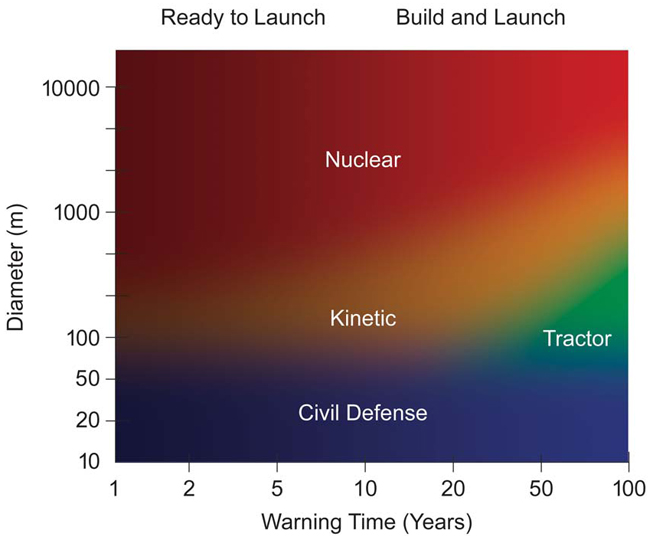
Source: the NEOShield Project

The figure above shows the amount of time that we need to know ahead given an asteroid’s size and the most likely way to prevent collision. For the fastest deployment, as suggests by the graph, the fastest would be a nuclear warhead, followed by a kinetic impactor and lastly the gravity tractor. From a cost point of view, the cost of sending each object into space would be around the same, but the cost of building each one ranks (from most expensive to cheapest): nuclear bomb, gravity tractor (which is just a satellite), and kinetic impactor (an object with a propeller). Under these criteria, the kinetic impactor is the most cost-effective with moderate time-constraints and moderate asteroid sizes. The major drawback for gravity tractors is that it takes too long for the effect to take place, and it requires an extremely accurate location of the asteroid and maneuvering of the satellite to put it in an optimal position for using gravitational force to redirect the asteroid. However, to be able to obtain the location information is far beyond any form of accurate sensor range in our current state of technology and can only yield estimates, which do not provide adequate intelligence for effective gravitation. For nuclear warheads, there is the problem of safety and post-blast repercussions. If the asteroid just happens to have a fault running through the middle (as dramatized in the film Armageddon), the blast and shockwave that comes from the bomb would cause the asteroid to split into two large pieces and create even larger destruction. For a kinetic impactor, as supported by the calculations we made in the data section, as long as the impactor is moving at a sufficient velocity (which can be achieved with ease due to the lack of friction in space), it can successfully cause an asteroid of any size to miss Earth, given enough distance and time between the Earth and the rock.

The Answer

After evaluating the three methods of preventing collision, kinetic impact is certainly the most cost-effective. It must be said that in terms of pure effectiveness, a nuclear detonation would have the most impact on the asteroid, but there are too many political implications and destructive consequences that come with nuclear explosions. For the cleanest and safest method, gravity traction is most preferable, but due to the lack of technology and accurate information, it is no doubt the least effective, not to mention the amount of time and effort needed to ensure the most effectiveness (already insignificant compared to kinetic impact and blast deflection) that it will have upon the asteroid.

What Did We Learn?

Even though preventing a world-wide catastrophe caused by an asteroid sounds like a big deal (which it really is), the science behind the idea of pushing an asteroid away is really based on simple classical physics principles (mostly Newton’s Second Law). Through this project, we were able to learn what people on Earth would have to do to avoid asteroid collisions and the amount of efforts needed in order to achieve safety. Through calculations, we learned just what magnitudes that we will be dealing with when it comes to asteroids and potential elimination of the human race. By doing this project, we also acquired skills of modeling and applying what we have learned before in physics to novel situations such as the one we wanted to investigate.

If We Were to Do This Once Again:

For the demonstration that we filmed, we would definitely change the components. The surface we used had a lot of friction (pool table) even though it gave a lot of control in terms of the direction the ball rolled in. Additionally, we would like to try to have a moving kinetic impactor representation to create a demonstration closer to the actual situation of kinetic impact on an asteroid. It would be nice to be able to use metal ball bearings on a slippery surface to represent the asteroid and impactor and minimize friction.

Group 2 Project Conclusion

What were our results, and what do they mean?

Acoustic Flute Acoustic Guitar Acoustic Piano Analog Synthetic Flute Analog Synthetic Guitar

analog synth piano final FM Synthetic Guitar FM Synthetic Piano


Instrument

RMS Error

Acoustic Flute

0.3632

Analog Synthetic Flute

0.2644


Acoustic Guitar

0.3104

Analog Synthetic Guitar

0.2178

FM Synthetic Guitar

0.2505


Acoustic Piano

0.3342

Analog Synthetic Piano

0.2875

FM Synthetic Piano

0.2272

The Root Mean Square Error method shows the difference between data points and a mathematical model. In this case, the RMS is showing the different between the synthetic and acoustic waves and a sine curve. As can be seen in the table above, our data clearly shows that acoustic waves do not fit a mathematical model as well as synthetic waves. The average of all synthetic waves’ RMS errors (including FM waves) was .2495, while the average of acoustic waves’ RMS errors was 0.3359. This means that the synthetic waves were more regular; this is understandable because there is no natural pitch and volume variation in a computer-generated wave.

 Were our results as predicted? Why or why not?

Our earlier post about expected outcomes reveals that we had some misconceptions about sound waves, especially synthetic sound waves.  We were correct in predicting “more organic” waves for instruments. However, we misunderstood “more organic” to be a simple sine wave. We imagined a “natural” sine wave to have nice curve with a consistent frequency. On the other hand, we thought the synthetic wave would be more sharp and geometric looking. In reality, both acoustic and synthetic waves are sawtooth waves for the instruments that we were analyzing.

Synthesizers cannot reproduce the natural amplitude or pitch variation that occurs with acoustic instruments. When people play instruments they cannot sustain a note at the same volume with the precision that a computer program can. Especially in the case of a guitar or a flute, the pitch may also vary slightly based on how the person is playing. In the case of a guitar the pitch could change based on finger placement, with the flute based on lip shape. After researching how sound waves are produced by synthesizers and instruments we have realized these misconceptions. We are using the scientific information outline below to analyze our data.

What science did we learn during this project?

An Introduction to Overtones, Harmonics, and Additive Synthesis (from “Synth School,” CreativeCommons):

This project allowed us to learn about the way sound waveforms are produced naturally by acoustic instruments, and how synthesizers attempt to replicate these waveforms. We learned that waves produced by acoustic instruments are a result of the various overtones and harmonics unique to each instrument. These harmonics cause interference; the waveforms are distorted from the pure sine wave shape. We learned that different instruments naturally produce different sets of overtones as a result of their shape. For example, a clarinet is known to have a square waveform, which results from the instrument only producing the odd harmonics.The shape of an instrument determines its unique set of harmonics. Closed tube, cone-shaped, and string instruments (and the various instruments within each of those categories), will all have different sets of harmonics. The three instruments we worked with, though each having a unique series of harmonics, all naturally produce a sawtooth waveform.

A wave progresses from a sine wave to a sawtooth form as more harmonics are added.

(from TeachNet Resources, http://resources.teachnet.ie/amhiggins/squaresaw.html)

The biggest factor that affects the “natural” quality of an acoustic instrument is the variation in pitch and amplitude, which cannot be readily replicated by a synthesizer. Synthesizers tailor their replications of each sound by trying to use the same set of harmonics produced naturally by each instrument. For example, a synthesizer will try to replicate the sound of a clarinet by adding only the odd harmonics onto the fundamental tone, just as would happen with an actual acoustic clarinet. The synthesizer’s cold, unnatural sound is the a result of the lack of variation found in acoustic tones.

The set of harmonics produced will differ from instrument to instrument, and those unique sets of harmonics are the information used by synthesizers to try to replicate the unique sound of the individual instrument. Thus, the wave shape of a tone of an individual instrument will be the same whether synthetic OR acoustic. The differences between synthetic and acoustic tones, then, lie in the variations produced naturally in pitch (frequency) and volume (amplitude) of an acoustic instrument.  


What would we differently if you had to do this project again?

If we had to do this project again, we would approach it very differently given the knowledge we have now. We would do more preliminary research before even starting our data collection. In addition, we would take our data in an environment with minimal ambient sound and controlled conditions (like temperature which might have affected the pitch, etc. of our acoustic instruments.) Another thing we would have to do before data collection is become more acquainted with our LabQuest! After taking our first set of data, our LabQuest would not transfer any data to a computer, and then deleted our data altogether. Testing our LabQuest before taking significant amounts of a data is a step we would take at the very beginning of our project if we had the opportunity to start from scratch.


What would we do next if we had to continue this project for another 6 weeks?

If we had to continue this project for another six weeks, we would test out other synthesizer programs (other online programs like AudioSauna, maybe iPhone applications, or look at more expensive programs) to see if the effect is consistent among all synthesizers. We would expand our project to include other instruments as well, apart from piano, guitar, and flute. In taking our data, we would try to take more data samples per second (although that might include using a more sophisticated device than a LabQuest), so as to hopefully obtain more accurate waveforms. On the AudioSauna program that we used for our project, there are certain features which allow for manual changes in wave shape and harmonics added to a tone. We would like to see if we adjust these features, if we might be able to more accurately replicate the natural waves of the acoustic instruments.

In addition to taking more data, we would consider expanding our project to have a more interdisciplinary approach. We would like to incorporate Media Studies into our project, and look at how prevalent purely synthetic tones are found in today’s recorded music. Also, we are interested in expanding our project in a psychological context as well, to see if humans are able to tell the difference between an acoustic and a synthetically produced tone.

Finally, if we had another six weeks to work on this project, we would devote much more time to research and learning about the process of sound synthesis and how more complicated and variable waveforms are created with acoustic instruments. More knowledge on the subject would help us analyze our data much more accurately, and see the differences and subtleties in all of our data.


Group 6 – Analysis and Conclusion

Plan

Our goal in pursuing a project with NFC devices was to further understand the technology and to see if we could amplify the signal of NFC devices to boost the range of data transfers. We planned to do this by inserting thin sheets of metal with high magnetic permeability between the NFC device and a regular metal object, which under normal circumstances grounds the magnetic field and makes data transfers impossible. When we were unable to acquire the appropriate materials to do this testing, we pivoted our focus to testing how placing an NFC chip (tag) on materials of varying electromagnetic permeability affected the range of NFC transfers. We predicted that when placed on an object with high permeability like ferrite, an NFC tag would be capable of transferring data at greater distances than when placed on objects of lower permeability.

Testing

To test the effect of a material’s permeability on the range of the transfer, we first looked at the range at which data transfer was possible without backing. Using a ruler, we measured the distance between the NFC tag and the NFC reader device. The NFC reader reader device was a NFC tag powered by the battery of a smart phone. We did several trials to establish an average distance for data transfers when the standalone NFC tag had no backing. In each test, we moved the NFC reader from out of transfer range towar the NFC tag until the rader device registerd the NFC tag, signifying a data transfer was successful. We then measured the distance between the reader device and the NFC tag when transfer was established. This operation was then repeated with different backing materials.

Results

We found an average of 3.645 cm for data transfer to be possible when the NFC tag had no backing. Data transfer between the NFC tag and the reader was impossible when the tag had a stainless steel backing. Trials with a 10 cm iron backing showed a smaller range of data transfer with an average of 1.72 cm.  We then found an average of 4.115 cm for a 1.2 cm glass backing, 1.98 cm for a 16 mm ferrite backing and 3.325 cm for wood backing. Interpretation We hoped that our testing would show a positive correlation between permeability and range of data transfer. These hopes were burned to the ground after several rounds of testing with different materials, when it became clear that our data was inconsistent with average permeabilities of our materials.

Materials Avg. Permeability Avg. Range for data transfer
Vacuum π4E-7   (1) Untested
Air 1.2566375E-6   (2) 3.645cm
Wood 1.25663760E-6   (3) 3.325cm
Iron 6.28E-3 1.72cm
Ferrite >2.0E-5 (varied depending on composition) 1.98cm
Glass 4.86E-15 4.115cm
Austenitic Stainless steel  1.05-1.1 No transfer

We hypothesized that greater permeability would ad to greater transfer distance, but as the test results show, our data was completely unpredictable. For example, when testing with the permeable metals iron and ferrite, we expected to see a greater transfer distance when the NFC tag was placed on ferrite, the permeability of which is on average far higher than most iron. Additionally, though non-magnetic materials like wood, glass, and air would normally be expected to achieve similar averages, tests with glass produced a surprisingly higher average of data transfers than the other nonmetal materials. Austenitic stainless steel backing didn’t allow data transfer because it is non-magnetic.

Analysis

What can account for these inconsistencies in our results? Unfortunately, there were too many uncontrolled and unknown variables that could have affected our tests to provide any one specific explanation. The quality and composition of metals used in the tests are unknown; ferrite, for example, has a wide range of permeability depending on the ratio of its components. Purity of iron affects its permeability as well, and there are a variety of stainless steels with variable permeability. Permeability is also affected by temperature, and our inability to control the temperature of the test area could have accounted for statistical discrepancies. Human error in the form of misreading a taken value or changes in how the NFC tag was held are also possible sources of confusing data.

Science

We were able to learn about the technology that powers NFC transfers in our research and experimentation, as well as the differences between NFC and similar wireless transfer technology like RFID. We also learned about electromagnetic permeability. Unfortunately, we did not find that in specific cases permeability affected the electromagnetic field of the NFC chips in a meaningful way.

Next Time

If we were to conduct this experiment again, we would acquire materials from sources that provided details on the composition of said materials in order to properly ascertain their actual permeabilities. Ideally we would be able to acquire thin foils of permeable metal so we could follow up on our original plan of adding a thin layer between the NFC tag and a grounding metal object. If we had another 6 weeks, we could attempt to build a rudimentary signal amplifier by altering a ham radio (suggestion courtesy of Larry Doe).

References

  1.  Definition of permeabilty in a vacuum
  2.  B. D. Cullity and C. D. Graham (2008), Introduction to Magnetic Materials, 2nd edition, 568 pp., p.16
  3.  Richard A. Clarke. “Clarke, R. ”Magnetic properties of materials”, surrey.ac.uk”. Ee.surrey.ac.uk.


Group 4 Conclusion

What were your results?

  • All the trials-including the RF meter trial-demonstrate the highest amount of readings 1 meter away from the wireless access point (WAP), and as expected, all three trials show a negative association between distance and dBm. As previously mentioned, these are the circumstances for each of the trials:

  • Trial 1: WAP uncovered.
  • Trial 2: WAP covered with cinder block.
  • Trial 3: WAP covered with cinder block and surrounded by 12 wood planks.
  • Trial 4: RF electrosmog meter used, WAP uncovered.

Descending Values

  • We expected the signal strength to descend from Trial 1 to Trial 3, but instead, Trials 2 and 3 alternated in dominant strength between distances. There was an even split in averages, with 5 distance points of Trial 2 dBm readings being greater than Trial 3 dBm, and with 5 distance points of Trial 3 dBm readings being greater than Trial 2 dBm readings. Because of this even split, we are hesitant in reporting that increasing the volume of medium to an already-covered WAP decreases the signal strength.

  • A peculiar observation to note is that from 2 meters, trials 2 and 3 gave dBm readings that were significantly lower than the data of trial 1. Trial 1 at 2m yielded an average of -41.6dBm, while Trial 2 yielded -49.4dBm and Trial 3 yielded -50.6 dBm. The 2m was the distance that showed the largest gap in signal strength between Trial 1 and 2-3. Continue reading

Group 3 – Conclusion

After careful examination of our data, it can be concluded that increasing screen brightness does increase the power consumption of a laptop. However, while we hypothesized that changing the brightness would increase power consumption by a consistent ratio, we found no such consistency. In our data, we calculated that increasing brightness from 25%-100% increased wattage consumption by an average of 26%, but there were great deviations within this percentage. This was calculated by subtracting the wattage consumption at 25% brightness from the wattage consumption at 100% brightness, and dividing that number by the max wattage consumption.


Example Calculation for MacBook Pro (mid-2012, 15 inch w/ Retina Display):

18.5W-11.2W = 7.3W/18.5W= 39% decrease in power usage.

All the calculations were averaged together to receive a value of 26%.


This inconsistency may be due to several possible sources of error, including the running of background programs that we were unaware of, which could create a second variable affecting the recorded power values. Another possible source of error is equipment failure (as observed in Tori’s data but to a lesser, less noticeable degree). Our results show that, while decreasing the screen brightness of a laptop may decrease the power output of the computer, the decrease is slight and inconsistent.

The science we learned during our experiment included a fuller understanding of the scientific method, data collection methods, and data analysis through graphs. We also gained a better understanding of the relationships between voltage, current, and power, including V=IR (Ohm’s law) and P=IV.

If we conducted this project again, we would try to take more data points from many more laptops to create a broader relationship between screen brightness and power output. We would make more of an effort to control for accidental variables, like background programs. We would also start our research earlier, to give ourselves more time to collect more data and analyze it more thoroughly using LoggerPro.

If we were to conduct our research for 6 more weeks we would take data from many, many more laptops and we would expand our research to include laptops of other brands, like Toshiba and Sony, instead of limiting ourselves to only Apple laptops. We could also expand our data collection techniques to include other screen brightness levels, instead of only taking data at 4 different brightness levels. If we had more time, we would also closely examine the laptops with high power output to see if they were infected with viruses. This would provide a bigger picture of the relationship between screen brightness and power output.


Group 2 Project Data

How did we take our data?

Using a LabQuest, with microphone and sound level meter sensors, we recorded a single tone (of the musical note C), played by each instrument: piano, flute, and guitar. We also recorded tones (again, the note C) created by two different synthesizer programs: one an FM synthesizer, and one an Analog synthesizer. Our data tables are not posted here on the blog, as each table would have around 500 points of data. Instead, below is our data represented in graphical form created by LoggerPro. 

All of our data was taken in the same, quiet environment with the hopes of minimizing ambient noise. We used a Steinway piano, a Yamaha flute, and a Taylor guitar. We used a free online program, called AudioSauna, which provided us with the synthetic tones we needed for each instrument, both FM and Analog.

Given that the known frequency of the note C is around 261.6 Hz, we took our recordings at a rate of 500 samples per second. We first attempted to record at a rate of 1000 samples per second, but we were limited by the capabilities of our LabQuest. Therefore, the graphed waveforms from our recordings may not represent the subtleties in the differences between acoustic and synthetic (both analog and FM) waveforms. 

In general, the graphs of the synthetic tones– but especially the FM synthetic tones– showed more uniform waves relative to those of the acoustic tones. The acoustic tones seemed to form a sort of pattern over time, with more variance in the sound pressure. These patterns and variance may be caused by interference of the different harmonics that constitute the tones of acoustic instruments. The LabQuest and LoggerPro did not give default units for Sound Pressure, but deemed them as “arbitrary.” 

More details and analysis to come on Friday!


PIANO

Acoustic Piano

Acoustic Piano


Synth Piano

Analog Synth Piano


FM Piano

FM Synth Piano


FLUTE


Acoustic Flute

Acoustic Flute


Synth Flute

Analog Synth Flute


GUITAR


Acoustic Guitar

Acoustic Guitar


Synth Guitar

Analog Synth Guitar


FM Guitar

FM Synth Guitar


Group 3 Graphs

We graphed the output of power, current, and voltage for each laptop computer we received data from. We excluded all zero values, as we attribute those recorded values to a malfunction in the Watts Up Pro or human error while recording data. We can see from our graphs that power and current increase, if only slightly, when the screen brightness is increased. The voltage, however, does not seem to change much and does not have an overall trend of increasing or decreasing when the screen brightness was changed.

Picture 6 Picture 8 Picture 10

6 – Data Update

Our project started ambitiously with the goal of amplifying NFC signals, or reversing the nullification of NFC that occurs when a chip is backed with metal. Unfortunately we could not acquire thin enough materials (such as permalloy or ferrite foil/film) to properly test whether this was possible. We then pivoted and decided to test the range of data transfers when the NFC chip was backed with various materials of different electromagnetic permeability.

+-+-+-+-+-+-+-+-+-+-+-+-+-+-+-+-+-+-+-+-+-+-+-+-+-+-+-+-+-+-+

Establish an average distance of transfers from

Samsung NFC NFC on Li-ion battery
to
3.8cm Circular RapidNFC NTAG203
with
no backing


Trials

  1. 3.5cm
  2. 4.0cm
  3. 3.7cm
  4. 3.7cm
  5. 3.8cm
  6. 4.0cm
  7. 3.7cm
  8. 3.5cm
  9. 3.3cm
  10. 3.8cm
  11. 3.6cm
  12. 3.8cm
  13. 3.3cm
  14. 3.9cm
  15. 3.5cm
  16. 3.8cm
  17. 3.9cm
  18. 3.3cm
  19. 3.3cm
  20. 3.5cm

Avg. 3.645cm

+-+-+-+-+-+-+-+-+-+-+-+-+-+-+-+-+-+-+-+-+-+-+-+-+-+-+-+-+-+-+

Establish an average distance of transfers from
Samsung NFC NFC on Li-ion battery
to
3.8cm Circular RapidNFC NTAG203
with
.9mm stainless steel backing


Trials

  1. No Transfer
+-+-+-+-+-+-+-+-+-+-+-+-+-+-+-+-+-+-+-+-+-+-+-+-+-+-+-+-+-+-+

Establish an average distance of transfers from

Samsung NFC NFC on Li-ion battery
to
3.8cm Circular RapidNFC NTAG203
with
10cm iron backing

Trials

  1. 1.9
  2. 2
  3. 1.4
  4. 1.1
  5. 1.6
  6. 1.8
  7. 1.2
  8. 1.1
  9. 1.5
  10. 1.7
  11. 1.6
  12. 2.2
  13. 1.9
  14. 2.3
  15. 2.4
  16. 2.1
  17. 1.7
  18. 1.6
  19. 1.5
  20. 1.8

Avg. 1.72cm

+-+-+-+-+-+-+-+-+-+-+-+-+-+-+-+-+-+-+-+-+-+-+-+-+-+-+-+-+-+-+

Samsung NFC NFC on Li-ion battery
to
3.8cm Circular RapidNFC NTAG203
with
1.2 cm glass backing

Trials

  1. 4.1
  2. 3.5
  3. 3.7
  4. 4
  5. 4.5
  6. 3
  7. 4.2
  8. 4.3
  9. 4
  10. 4
  11. 4.1
  12. 4.7
  13. 4.5
  14. 4.1
  15. 4.2
  16. 4.2
  17. 3.8
  18. 4.3
  19. 4.5
  20. 4.6

Avg. 4.115cm

+-+-+-+-+-+-+-+-+-+-+-+-+-+-+-+-+-+-+-+-+-+-+-+-+-+-+-+-+-+-+

Samsung NFC NFC on Li-ion battery
to
3.8cm Circular RapidNFC NTAG203
with
16mm ferrite backing

Trials

  1. 2.1
  2. 2.4
  3. 2
  4. 1.8
  5. 2
  6. 1.9
  7. 2
  8. 2.2
  9. 2.4
  10. 1.7
  11. 2.1
  12. 1.9
  13. 1.7
  14. 2
  15. 1.5
  16. 1.9
  17. 2.1
  18. 2.0
  19. 1.8
  20. 2.1

Avg. 1.98cm

+-+-+-+-+-+-+-+-+-+-+-+-+-+-+-+-+-+-+-+-+-+-+-+-+-+-+-+-+-+-+

Samsung NFC NFC on Li-ion battery
to
3.8cm Circular RapidNFC NTAG203
with
Wood backing

Trials

  •      1.  3.2
  1. 3.2
  2. 3
  3. 2.8
  4. 2.9
  5. 2.7
  6. 2.4
  7. 3.6
  8. 3.8
  9. 3.4
  10. 3.6
  11. 3
  12. 3.9
  13. 3.7
  14. 3.9
  15. 3.3
  16. 3.5
  17. 3.9
  18. 3.5
  19. 3.2

Avg. 3.325cm

+-+-+-+-+-+-+-+-+-+-+-+-+-+-+-+-+-+-+-+-+-+-+-+-+-+-+-+-+-+-+


Group 3 Project Data

Model Power @ 25% Power @ 50% Power @75 % Power @ 100%
MacBook Pro (mid-2012, 15 inch w/ Retina Display
Volts 117 116.6 116.8 117.2
Amps 0.542 0.546 0.564 0.603
Watts 11.2 12.2 14.4 18.5
Apple MacBook Pro (13-inch, mid-2012) *Could this computer be affected by viruses?*
Volts 118.8 119 119.1 119.4
Amps 0.908 0.923 0.936 0.961
Watts 44.3 44.6 45.9 48.3
Apple MacBook Pro (13-inch, mid 2009)
Volts 119.3 119.1 119.2 119
Amps 0.54 0.544 0.555 0.582
Watts 10 10.9 11.9 14.4
MacBook Air (mid 2012, 13-inch)
Volts 117.3 117.3 117.1 116.9
Amps 0 0 0 0
Watts 0 0.1 0.1 0
MacBook Pro (mid 2012, 15-inch)
Volts 116.9 116.9 116.9 117.2
Amps 0 0 0 0
Watts 0.1 0 0 0
MacBook Pro (mid 2012, 15 inch)
Volts 117 117.1 117.2 0
Amps 0 0 0 0
Watts 0.1 0.1 0 0
MacBook Pro (2010, 13-inch)
Volts 115.8 115.9 116 116
Amps 0 0 0 0
Watts 0 0 0.1 0
MacBook Pro (mid-2012, 13-inch)
Volts 115 115 115.3 115.2
Amps 0 0 0 0
Watts  0  0  0 0
MacBook Pro w/retina (mid-2012, 13-inch)
Volts 115.3 115.4 115.4 115.4
Amps 0 0 0 0
Watts 0 0.1 0 0.1
MacBook Pro (late 2011, 13-inch)
Volts 115.4 115.4 115.3 115.4
Amps 0 0 0 0
Watts 0 0 0.1 0
MacBook Pro (13-inch, summer 2012)
Volts 115.4 116.6 116.2 115.6
Amps  0.556 0.578 0.582 0.587
Watts 8.8 9.8 9.4 12.5
MacBook (summer 2008, 13-inch) *Molly’s Computer Exhibits Very High Power Usage. She may want to check for viruses.*
Volts 115.6 115.5 115.6 115.7
Amps 0.641 0.655 0.668 0.685
Watts 44.4 46.6 47.1 55.3
MacBook Air (summer 2012,13-inch) *High Power Usage*
Volts 116 115.9 115.9 115.7
Amps 0.43 0.733 0.739 0.745
Watts 32 51.6 52.2 52.7
MacBook Air (summer 2012, 13-inch)
Volts 115.6 115.7 115.6 115.7
Amps 0.373 0.368 0.337 0.384
Watts 24.6 26.6 26.6 28.3
MacBook Air (mid 2011, 11-inch)
Volts 116.7 116.6 116.7 116.9
Amps 0.536 0.543 0.549 0.561
Watts 9.9 10.7 11.2 12.9
Every Laptop that we tested is some variation of Apple’s MacBook Pro or MacBook Air. Since Apple does not have specific “model numbers” for their laptops, we indicated the time that the laptop was released and the size of the screen. The data was taken using our Watt’s Up Pro’s supplied by Prof. Magnes. Electrical power is measured in wattage, which is equal to the voltage (volts) multiplied by the current (amperes). Amps are equal to the amount of electrical charge passing through a circuit per unit of time, with 6.241x 10^18 electrons per second being equal to one ampere.  We measured the watts, amperes, and volts of each laptop with screen brightness at 100%, 75%, 50%, and 25%. Each laptop had every application closed except for Safari’s homepage, which was what was on the display for every measurement. There are some glitches in the current data. Tori’s Watt’s Up Pro gave measurements of approximately 0 for both amps and watts for a reason that is still under investigation. It is possible that the device was not configured correctly for reading current, as power = voltage x current, and a zero value for current would cause a calculated wattage to be zero as well. Some laptops, including Molly’s 2008 MacBook and the 13-inch mid 2012 MacBook Pro gave very high readings for watts and amps. We are considering possibilities for this outlying data, including the chance that viruses are causing the computers to run less efficiently or dysfunctional batteries. We will graph the data for each type of laptop, but it is clear from our data tables that increasing brightness consistently increases power usage. This is consistent with our original hypothesis. Amps also increase consistently, but voltage does not vary directly according to screen brightness. This makes sense since voltage is only the electric potential difference between two points.References:

December 2010 – By Steven S. Zumdahl, Susan A. Zumdahl – Brooks/Cole, CENGAGE Learning – 2010.12.17 – Hardback – 1,038 pages – ISBN 0840065329

Group 1: Update on Data Collection

There have been many bumps along the road to completing this project. What began as an investigation of wireless power transmission by using the market’s current wireless charger pads, became an investigation on the science behind how wireless charger work. The pad we originally ordered was out of stock, which pushed our schedule back. Then the charger that we ultimately received came without the inductive phone case, again this caused a change in our plans. We then decided to collect data on the magnetic field produced by the charger pad, and to our surprise there was no magnetic field. We researched why there was no magnetic field and we found that without the inductive case no field would be produced. What follows are the applications of this technology and an explanation of how it works.

What is wireless power transmission:

At the turn of the century Nikola Tesla suggested and demonstrated the idea of wireless power transmission. Today this technology can be seen in different facets of our lives, some examples are wireless phone charges and many electric toothbrushes. Today there are hopes to expand the uses of this technology, some major names in this field are the Wireless Power Consortium and WiTricity. The Wireless Power Consortium is attempting to universally standardize qi (chee) technology, which is the technology used for wireless power transmission. Though the industry is currently small there are hopes to make wireless power transmission as widespread as wi-fi is today, and eventually be used in our daily lives in ways such as household appliances. Currently the industry is limited by the wireless range which is on average 5 millimeters to 40 millimeters and it is used on devices that use up to 5 watts. WiTricity which was created by MIT is currently trying to increase the wireless range as well as the device wattage.

How does it work:

The way that wireless conductivity works is that there are two coils, one transmitter and one receiver. A current is run the the transmitter coil which creates a magnetic field. When the receiver coil is place within the magnetic field parallel to that transmitter coil then a charge is induced in the receiver coil, which can be used to power LED lights or charge phone batteries. It was because of the simplicity of the process that we believed that we could measure the magnetic field produced by the transmitter even without the receiver. The problem is that the devices on today’s market are not as simple. What we were missing was the receiver which turned out to be the most important part of today’s wireless charger. Within the charging receiver case there is a circuit board which is connected to the coil. The circuit board was two main components, a radio transmitter and the load which regulates the power supplied to the phone. The load uses the transmitter, which operates by sending unidirectional signals via back-scatter modulation to the transmitter pad. The load communicates how much power is needed, this allows the pad to turn its magnetic field on and off depending on whether the phone is fully charged or not. This is why we were unable to calculate the magnetic field because it was not receiving any signals to broadcast its magnetic field.

Phone case with coil and circuit boardIMG_1276IMG_1264IMG_1263


Bibliography:

“Chapter 2 Synchronous Rectification.” Thesis. Virginia Tech, n.d. Chapter 2 Synchronous Rectification. Web. 4 Oct. 2013. <http://scholar.lib.vt.edu/theses/available/etd-173510281975580/unrestricted/chapter2.pdf>.
The Fundamentals of Backscatter Radio and RFID Systems. Disney Research, Pittsburg, 2009. Web. <http://wireless.vt.edu/symposium/2009/2009Tutorials/Fundamentals%20of%20Backscatter_Part%202_Griffin.pdf>.
“Inductive Charging Transmitter.” China (Mainland) Inductive Charging Transmitter Export on Wholesale Market Exportmarkets. Sunshine Good Electronics Company, n.d. Web. 04 Oct. 2013. <http://sunshine-good-electronics-company.exportmarkets.com/product/71613/inductive-charging-transmitter>.
“INTEGRATED WIRELESS POWER SUPPLY RECEIVER, Qi (WIRELESS POWER CONSORTIUM) COMPLIANT.” Texas Instruments. Texas Instruments, Mar. 2012. Web. 4 Oct. 2013. <http://www.ti.com/lit/ds/symlink/bq51013a.pdf>.
“An Introduction to Wireless Charging: Changing the Way We Think about Power.” An Introduction to Wireless Power. Wireless Power Consortium, n.d. Web. 04 Oct. 2013. <http://www.wirelesspowerconsortium.com/what-we-do/how-it-works/>.
Yates, Alan. “Wireless Power Experiments.” Alan’s Lab. N.p., 26 Apr. 2011. Web. 29 Sept. 2013. <http://www.vk2zay.net/article/253>.