Alex Molina & Kadeem Nibbs
Computational Physics 375 – Final Project

Project Motivation

We wanted to model the Long Jump track & field event to see if we could mathematically incorporate technical elements to the simple projectile motion model and see tangible differences in jump distances.  We also wanted to model the effects of air, since we thought that wind speed and air density must have some effect on jump distances, but did not know how to quantify its impact.  We believed we could achieve these goals with a comprehensive Matlab program, and Chapter 2 of Giordano and Nakanishi’s Computational Physics on realistic projectile motion gave us a clear starting point.

Program Description

This program simulates the long jump track and field event to observe changes in jump distance as related variables are adjusted. The variables we were most interested in are: air density, to determine if jumps done at different altitudes are comparable; wind speed, to observe how much wind resistance can affect performance; whether or not the athlete cycles his or her arms in the air, to see how this movement affects body position in the air; and, of course, the final jump distance.  We could also adjust the size of our athlete using our program, but the adjustments, as long as they are kept within reasonable limits, would have a negligible effect on the results.  The athlete’s physical proportions are based off of our very own Kadeem Nibbs, who always wanted to participate in the long jump but never could due to scheduling conflicts.

We originally wanted to use 3D models to run all of our tests, but working with 3D shapes and deforming them proved difficult.  We decided to use point particles for the tests where they provide an accurate approximation (wind assistance and air density), and then 2D “patch” shapes for tests where body position became exceedingly important (limb cycling).  For the trial where the athlete did not cycle his limbs, we created one fixed-shape rectangle to model the athlete’s body, as if he were held rigid throughout the entire jump. We modeled the athlete with two rectangles when limb cycling was allowed, one rectangle to represent the torso, and another for the legs, so that they could move independently.

Final Results

Real World properties and their affect on Long Jumping:

While our preliminary results showed that wind had a major impact on the final jump distance, with a difference of 7m/s resulting in a change of approximately 2 meters in jump distance, we found that this was due to a missing square root sign when calculating velocity.  When this was fixed, we found that the same difference in wind speed accounted for a difference in inches in jump distance.

Our Resulting Projectile Motion with Varying Wind Speed:

Our Resulting Projectile Motion with Varying Wind Speed (close up view):

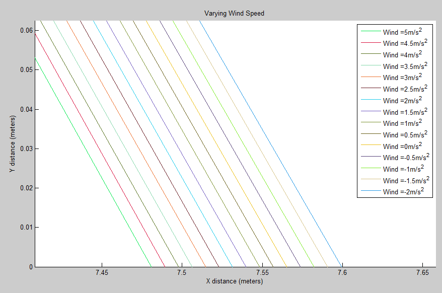
A 0.1 change in meters is about a difference of 4 inches. While this may seem negligible on a macroscopic level, the top two World Records in the long jump only differ by 4.5 inches.  So a fortuitous wind gust may be the difference between a gold medal and nothing.

For our second real world property we found that air density had a negligible effect on the jump distance, as variations of up to 50% in air density resulted in less than a millimeter of difference. This reaffirms what was learned in introductory mechanics: that air resistance is negligible in most cases of projectile motion, with exceptions being when the air is moving and when the object is moving at high speeds.

Our Resulting Projectile Motion with Varying Air Density:

Air resistance will not significantly affect an athlete jumping at 20mph into still air. This also shows that although air density can be as high as 1.2kg/m^-3 at cities near sea level, and as low at .75kg/m^-3 at cities 5000m above sea level, long jumps performed at any city in the world can be compared because of air density’s negligible effects on performance.

Modeling the Human with the Patch Mechanism:

After thoroughly researching track and field coaching manuals and websites, we learned that the purpose of cycling one’s arms and legs while in the air is to keep one’s torso from rotating forward. The torque generated during an athlete’s takeoff typically generates a large forward angular momentum. As a result, if an athlete does not cycle their arms/legs properly while midair, they may end up tilting too far forward, hitting the ground face first, and losing some of their teeth. This is demonstrated in the figure below when our code is run.

Our Resulting Projectile Motion Modeling a Human without limb cycling (head diving):

The forward angular momentum is especially detrimental because, if the torso is angled too far forward during the jump, the legs will inevitably end up far behind the body.  Since jump distance is recorded at the furthest back mark in the sand, if the athlete’s feet strike the ground a meter behind his center of mass, he is effectively disqualifying himself from competition.

By cycling his arms and legs, the athlete creates a forward angular momentum that is hopefully as large as that of his torso.  Since angular momentum is conserved for a projectile not subjected to any external torques, this generated angular momentum is subtracted from the torso’s angular momentum, allowing the athlete to stay upright.

Our Resulting Projectile Motion Modeling a Human while limb cycling:

In this upright position, it is easy to tuck the legs in front of the body, so that the hips are the first to strike the ground.  With this change in technique, we noted a difference of approximately 1.5 meters in the final jump distance.

Future Goals and Endeavors:

Continuing with this work, we would like to get a more holistic model of the long jump, as the run preceding the takeoff, which we entirely ignored, is an essential part of the event.  We would like to see how the approach speed to the jump affects the optimal takeoff angle, and also incorporate arms and more realistic body proportions for our athlete. We believe that this project has a future where a variation of our code could be used by coaches and athletes to see what a human body’s characteristics must be in order to have the most efficient and longest jump. This could mean studying how a different weight, speed, height, cross sectional area, etc. could produce the “perfect conditions for jumping the longest.”

Overall, we were able to model a human figure using the patch mechanism and we were very satisfied with this result. We were able to work together on close to 400 lines of difficult computational code and our knowledge of physical and computational concepts has since grown. We see now how realistic models can be designed on MatLAB and through this, they could be studied to see how different human characteristics could affect a long jumpers distance, whether it be a few millimeters to a few inches.

Our Final Computational Codes: 

Our final MatLAB code with and without the added patch motions are uploaded on this drive (just click the image below). Note that all the codes are listed in a text file (such as Notepad for Windows).  They will have to be manually copied into a script function in the Matlab program. This is due to the fact that we used a Citrix XenApp that allowed us to run MatLAB on our computers but not be able to save the files onto our own desktop.

References:

Knight, Randall Dewey. “Rotation of a Rigid Body.” Physics for Scientists and Engineers: A Strategic Approach. 3rd ed. Boston, Mass.: Addison-Wesley, 2012. 312-387. Print.

Giordano, Nicholas J., and Hisao Nakanishi. “Chapter 2: Realistic Projectile Motion.” Computational Physics. 2nd ed. Upper Saddle River, NJ: Pearson/Prentice Hall, 2006. Print.

MATLAB R2014b by MathWorks®

Acknowledgements:

We would like to thank Vassar College for allowing us to use their 24/7 Physics department computer room to help complete our project.  We would also like to thank our peers for giving us feedback on how we could expand on our project and helping us with fixing some minor computer codes. And a final thank you to Professor Magnes for teaching us the essential basics to coding and for guiding our project to what it is today. It has been a wonderful semester and we know that we will use our computational knowledge to further our intellect as physicists.

However entertaining modeling a drunk student back home after a long night may be, there is a physical system that corresponds to this movement. For example, gases and liquids both move according to Brownian motion. Brownian motion is the movement where molecules are free to move throughout their container. This movement is both based on random movements and on collisions with other molecules within the container. When looking at one molecule of gas or liquid, this movement appears completely random.

Although my programs model the motion of a wasted student, this random motion can be compared to Brownian motion easily. Not only that, but I can add additional and real physical variables to the code. I decided to focus mainly on drift. Drift for a drunk student can be thought of as a sober and conscious step towards their destination in addition to the random chance of stepping in that direction. This results in biased random motion, or random motion that is directed towards a specific region. In the college student’s case, it could be towards their room or a bathroom. Most Brownian motions in real physical systems include drift. Drift of gas can be caused by a temperature gradient, pressure gradient, physical force, or electromagnetic force.

My Matlab codes were designed to plot and determine the displacement squared of 3 different types of “walks.” The first is a very basic random walk. In this system, the walker has an equal chance of taking a step in the positive and negative x and y directions (Figure 1). This can be seen as a simplified system with completely homogenous conditions and one single molecule. The next system is a slightly more realistic system with more complicated and random directions (Figure 3). This is a better approximation for Brownian motion since it allows for the particle to move in any direction with a variable distance traveled for each time step. This also simplifies the system down to homogenous conditions. My final code is a manipulation on the first to account for drift (Figure 5).

 

Figure 1. Drunken Motion in 2D. No variables.

Figure 2. Statistics of Figure 1. Calculated with fitlm function of MATLAB.

Figure 3. Brownian Motion in 2D

Figure 4. Statistics of Figure 3. Calculated with fitlm function of MATLAB.

Figure 5. Drunken Walk with drift assigned with a 10% chance of taking 5 steps in +x or +y direction. fit=0.2550t^2+1.0161t+68.1101. R-squared=1.0000

 

Not only is drift visible on the motion map, the mean displacement squared is magnitudes larger between Figures 1 and 5. When drift was added, a second diffusion constant had to be added since the equation for mean displacement squared became parabolic. Since I am not comparing the mean squared displacements to a system with density (there is only one particle in my system), I can simplify the diffusion constants to be the slopes of their respective best fit lines. According to Figures 2,4, and 5, the diffusion constants are very precise and accurate (error is much less than 1% for linear diffusion), which indicate a statistically significant difference between the different walk methods.

The difference drift makes is considerable. This is important to keep in mind when considering chemical, biological, and physical systems. For example, a higher amount of drift, caused by a higher temperature or lower density on one side of a semi permeable membrane, alters solvent flux. Future directions for my experiment would be comparing the different sources of drift to each other. I would be very interested in modeling the real movement of solutes across a membrane under different gradients, such as temperature or solute density.

Figure 6. Brownian Motion in 3D. This isn’t all too significant to the rest of my project, but it is a visual representation of the path a liquid or gas molecule takes in a 3D homogenous box.

 

All 4 of my codes can be found here-https://docs.google.com/document/d/1nvyB5giUicIIiCJuKNKTwJagBlepP8J-IOQsMeMgB7Q/edit

The goal for our project was to develop an understanding of how physics methods can be used in the field of financial modeling. Primarily concerned with predicting prices and market shares over time, financial analysts have historically made liberal use of traditional physics and math techniques to best solve different sorts of systems.

A brief literature search indicated that one of the most commonly used physics tools in finance is the Monte Carlo method. Originally developed as part of the Manhattan Project to simulate the penetration of neutrons into a nucleus, the Monte Carlo method has come to refer to the general concept of using a massive amount of randomly generated numbers to simulate the development of a system based on some sort of probability distribution.

We began the project by familiarizing ourselves with basic Monte Carlo methods. First, we simulated the results of rolling two dice, simply generating two random numbers between 1 and 6 for an arbitrarily large amount of times. This basic method produced a distribution that described the most frequent combination of rolls. As expected, the mode of the distribution was 7. Next, we worked on a slightly more challenging problem, using Monte Carlo methods to numerically integrate a function. We used a rather trivial case, a circle inscribed in a unit square. The program dropped an arbitrarily large amount of points onto the system and counted how many fell within the bounds of the function. The ratio of this count to the overall number of points simulated the area of the function. The value of pi was obtained, confirming that our method was effective.

The next step was to decide which specific financial methods we would explore in depth. We decided to pursue two areas, the calculation of stock option prices and the evolution of the price of a good in a simple market over time.

A stock option is a financial tool used by traders to bet on the price of a stock over time. It allows the said trader, for a certain price, to be able to value the stock at a fixed price no matter how it changes in the overall market. A call option gives the trader the right to buy a stock at a fixed price over time, even when the market price rises significantly. Similarly, a put option gives the right to sell the stock at a fixed price over time, most useful when the stock price drops in the market over time. The problem in question is then to calculate the initial fee for which the trader can buy the right to have one of these options on the stock.

We explored three methods for pricing these options. The first was the Black Scholes method, which relies on knowing the values of several crucial parameters and the cumulative distribution that these parameters define. Equation for Black-Scholes where $C$ is the price of the option:

(1)  

where

(2)  

and

(3)  

$N(d_1)$ is the standard normal distribution of $d_1$ and $N(d_2)$ is the standard normal distribution of $d_2$ where $d_1$ and $d_2$ are a distribution.

 

This method proved to be rather rigorous as it necessitated at least basic knowledge of statistical modeling and the exact value of the parameters. The second method, the Monte Carlo distribution of pricing, was more elegant. It used a uniformly distributed set of random numbers between 0 and 1 and plugged the set into an equation that needed only the original price of the stock, the interest rate, and the volatility of the stock. Finally, the most elegant method to calculate the price of an option involved the use of binomial trees. Beginning with a strike price and a theoretical return on the stock, the binomial method calculated the value of the stock at an increasingly large number of nodes in the tree and then plugged these nodes into an equation that would value the price of the option.

The second system we studied was based off the Ising model used to simulate the evolution of a thermodynamic system over time. The most prominent application is the simulation of a ferromagnetic material whose constituent atoms possess spin characteristics that influence their neighbors. These spins naturally tend to align themselves in the same direction, and thus we have started with a ferromagnetic system in which all spins are aligned. We then simulate stochastic changes in the system that occur because of energy added by the temperature in a heat bath. As temperature rises, the greater there is that one of the spins will orient itself in a way that requires adding energy to the system. This is because the extra heat from the increased temperature supplies extra energy. The system is solved using a Monte Carlo method to calculate the probability of each atom flipping its spin per unit time, based on the interactions with its neighbors and the overall energy. The higher the energy, the higher the probability of flipping the atom. The average spin of the system is called the “Magnetization” and is a good way to represent how magnetic the metal is.

This system is then applied to the world of finance by simulating an evolving market of agents who can either choose to buy or sell a good, which is shown by:

(4)  

The decision to be a buyer or a seller influences the decisions of the nearest neighbors. However, all agents also are aware of a systematic trend in “magnetization” which in this case represents the price of the good in question. If there are more buyers than sellers, the price will be rising, so buyers will wish to join the sellers group to make a profit off of their good. The Monte Carlo method once again calculates the probability of these agents changing their identities, displaying the trend in price over time. The probability is given by:

(5)  

Then, the probability of an agent remaining/becoming a buyer is given by:

(6)  

(7)  

It is possible to see the stochastic nature of the pricing evolution over time, as well as the distribution of buyers and sellers in a market given some initial conditions. As we discovered, when buyers and sellers grouped with agents of their own identity, price is more volatile.

Below is a table that summarizes every method we have used, as well as providing the name of each file, found at this link https://drive.google.com/a/vassar.edu/folderview?id=0B01Mp3IqoCvhflF5azV4bHY2V0c3Vks0VXVyQkIxcnR4RmFaNDhVWEQtZGZSR2t6V2VWOHc&usp=sharing#:

 

Name of Method	Purpose	Name of Code
“Dice Roll”	Demonstrate the efficacy of a Monte Carlo method to simulate the distribution of a large amount of dice rolls	MonteCarloDiceRoll.m
“Numerical Integration”	Demonstrate how a Monte Carlo method could be used to calcuate unknown parameters from an arbitrary integral	montecarloexample.m
“Black Scholes Method”	Uses a set of parameters with known cumulative distribution to calculate the price of an option	BlackScholes.m
“Monte Carlo   Option Method”	Simulates the cumulative distribution from the Black Scholes method by creating a set of normally distributed random numbers that undergoes mathematical transformations	BlackScholes.m
“Binomial Trees”	Calculates the value of an option by valuing the strike price at various times based on a given interest rates. Assigns each of these values to a node in a tree and uses this structure to go back and value the option	BinomialTreesNThree.m
“Ferromagnetic Ising model”	Simulates the evolution of a ferromagnetic system in a heat bath by generating random numbers to calculate the probability of atoms in the system being either spin up or spin down.	IsingTest.m
“Market Strategy Model”	Applies the ferromagnetic ising model to a basic markets where agents that are either buyers or sellers replace the atoms. These agents follow the advice of their nearest neighbors or the tendencies of the market of a whole. These tendencies compete with each other and a Monte Carlo method simulates the probability of the agent choosing a strategy over time. The “magnetization” of this system, the average value of agents strategies, is a good way to represent the trend of the price of the good in the market.	TwoStrategyMarketModel.m

 

Project Discussion

Our goal for this project was to first model a two-body orbital system such as the Earth orbiting around the Sun using the Euler-Cromer method. The second goal was to model a three-body orbital system, such as the Moon orbiting the Earth while the Earth orbits the Sun.

We were successful in modeling a two-body system, and did quite a bit of work on studying the two- and three-body orbital systems. We tried both a computational approach and a numerical method to different ends. Ultimately, we determined that although the Euler-Cromer Method works is a good way to approach a two-body system, we were unsuccessful in modeling the three-body system using the Euler-Cromer Method.

First, it must be acknowledged that mass is never involved in the computational method. Honestly, we are not sure why, and that might genuinely be the source of the problem. The analytical method we used did need the masses and the sizes, and it worked much better, which raises questions about the computational method that we employed. If we were to incorporate mass into the computational method, however, we may have run into the issue that the sun is significantly more massive than the Earth. Had we attempted to base the movement of the Moon with an equation related to mass, the Moon likely would have jumped orbit from the Earth and gone to orbit the Sun.

Secondly, we would like to bring reference frames into the discussion. We did our project in the reference frame of the sun, but what would have changed if we were approaching the project from the reference frame of the universe? Or the earth? Or even the moon? — Because we approached it from the reference frame of the sun, any effect the earth and moon’s masses had on it would not appear in the simulation. We assumed that this is an acceptable assumption, because the relative masses would make it so that the effect of these two masses would negligibly affect the sun’s motion, but we are not sure if changing the reference frame would change the results.

The conservation of energy law requires the total energy of a closed system to remain constant. In an orbital system, if energy is positive or not conserved, the orbit can turn into a hyperbolic one instead of an elliptical.

In checking the energy of the systems: we first used the equation

(1)  

(2)  

Which comes from combining the orbital potential energy and orbital kinetic energy:

(3)  

But on second thought, $r<<R$ (where $r$ is the distance between the moon and the Earth, and $R$ is the distance between the Earth and the Sun). So we rewrote the energy of the moon as

(4)  

But strange “spikes” appeared in the energy plot, occurring where the radius changes dramatically. The energy plot is sinusoidal, completing one period in one orbit of the earth around the sun. We are not sure why this is so, but at second glance, the amplitude of the sine wave is very very small — it is between 4*10^44 and 4.5*10^44 Joules, so if we plot the energy from 0 the fluctuation is not visible.

Plot of Earths orbital energy for comparison:

Plot of Moon’s orbital energy:

This all raises the question: is the Euler-Cromer method inherently not useful for this problem? There is a good chance the program we wrote was the reason the simulation was unsuccessful. But what other reasons could there be for the program not to work? The Euler-Cromer is an iterative method, which makes a prediction on the next location based on the most recent information. It did work well for the two body system, producing a clean simulation of the Earth orbiting the Sun, which you can see below. (The simpler Euler method is not as viable of a method because over time the calculated information would get further and further from the “true” values, because it does not use the most recent information.)

So why is analytical easier, or at least more effective, in this case? The analytical is more specific than the computational method, because the motion of the system is already known and therefore the method can be tailored for the system. We as programmers are familiar with how and why the Euler-Cromer method works, and we are confident that this method is the best for our physical system. In the same manner, we are confident that our problem lies in how we are updating the x and y position of our orbiting bodies.

 

 

Link to analytical code:

https://docs.google.com/document/d/1mKmL4spylb1h6PttlyTBY9vIuZmfnLVQhfAzvSX2qBA/edit?usp=sharing

Link to Energy codes:

https://docs.google.com/a/vassar.edu/document/d/1KzZduXpxZ6-_gEja875FwCyn0Yvc_yO69JxQJSsasvA/edit?usp=sharing

https://docs.google.com/a/vassar.edu/document/d/15wfmgWwkx_TbmMf4Untcb5DXdADvH7mSrB8Vs2DKY4Q/edit?usp=sharing

Sushant Mahat

Mohammed Abdelaziz

Since last week, we have managed to greatly fine tune our program, and get more data.

We are using the same basic functions we created last week: TheInitiator and TheUpdater. However, as mentioned in the earlier post, our TheUpdater function was not functioning ideally. The profile of the Lennard-Jones potential is such that when two particles get close together (less than ~1.1 reduced unit in length), they exert a large repulsive force on each other and send each other moving away at large velocities. If you look at the Lennard-Jones potential in Figure 1 below, you can see that the force changes from attractive to slightly repulsive to extremely repulsive very fast (force changes by ~100 reduced units of force over ~0.3 reduced units in length). In real life, two particles repel each other before they get this close, so the force should never become very large. However, our function discretizes time, so there is a small chance that particles get very close to each other before they feel the repulsive force. This creates a repulsive force that catapults one of the particles, which breaks the law of energy conservation. The catapulting effect decreased when we decreased the time step dt (our discretization in time), but it did not go away completely.

To solve this problem, we divided TheUpdater into two parts: TheUpdater and TheEnforcer. TheEnforcer function calculates the force between each pair of particles and the total force on each particle. However, this function is designed such that if two particles accidentally get close to each other during dt, the force they exert on each other will be limited to a certain value (i.e. we cap the max force). We think this change is valid as two particles, with the velocities we use, would never get so close that they would exert more than our max force on each other. Apart from that, we have also made changes to the net force direction. In our last program, we were able to determine repulsive or attractive forces but it turns out we made an error in translating this information to force in the x direction and the y direction. This is especially hard as we have periodic boundary conditions, so it is not always clear whether a particle is “to the left” or “to the right” of another particle, for instance. However, we are confident that we have managed to get the force direction correct this time. We tested it by running a program with just 5 particles in a small box (size of 10* 10), so that it would be easier to monitor their interactions. During our several runs, we saw several different interactions where our particles curve around each other and attract at certain distances and then repel, as expected, which is a significant improvement to our last program. Video 1 showcases this test.

TheUpdater function now calculates positions and updates the velocity of our particle using the output from TheEnforcer. These data are fed into the main body script which calls upon another function: SpeedDist. SpeedDist finds the speed distribution of our particles. Figure 2 below shows that the average speed remains very close to 1 reduced speed unit, which was our initial average speed. In the coming weeks, we will also include another plot that shows the kinetic energy of all particles with respect to time, and the cumulative Kinetic energy of all particles. This information will be interesting because it can directly be used to calculate the temperature of the system, potentially allowing us to test the effects on the system when we manipulate the temperature.

Figure 1. This figure shows the Lennard-Jones potential. The x axis is length in reduced units. The reduced unit of length is based on the size of an argon molecule. The steep increase in potential below a distance of 1 suggests a rapid increase in repulsive force as two particles come close to each other. This essentially creates a “hard sphere” around each particle.

 

Figure 2. Speed distribution of 100 particles in a 25*25 box. The average speed remains roughly constant over the time interval and closely resembles Maxwell distribution. The total time for the simulation was 10 reduced time units where 1 reduced time units is approximately 2 picoseconds.

Video 1. This is a video of 5 particles in a  10*10 box. You can see the particles interacting in several ways.

Video 2. This is a video of 25 particles in a 10*10 box. It demonstrates that the interactions still work for greater numbers of particles (we have found that even simulations of 200 particles can be calculated in under a minute).

 

A note on reduced units:

Reduced units are used for convenience and simplicity in the equations used for the simulations because they avoid the need of having to put constants in every calculation. We have been somewhat vague about what each reduced unit represents in terms of common units, but will explicitly define these in a future post.

Edit (4/27/15):

We forgot to upload our most recent working script and functions; they can be found here.

For the second week of this experiment I chose to begin my analysis by focusing in on a topic I believe I’ve glossed over thus far: orbital resonance. What I have neglected to mention is that this “resonance” is a ratio of the orbital periods for two objects rotating around the same central body of mass, and is related to the orbital radii of the object.  To start with an example relevant to this project, the orbital period of an asteroid located at the 2/1 resonance point with Jupiter will be one half that of Jupiter’s, so it will complete two orbits for every one Jupiter completes. The relation between orbital period and orbital radii is given by Kepler’s Third Law, that the ratio

where P is orbital period and a is orbital radius is a proportion that holds for any object rotating around the Sun. This was used to calculate the location of the 2/1 resonance at 3.27 AU, knowing the orbital radius of Jupiter to be 5.2 AU and the using a ratio of periods as 2:1 for Jupiter:asteroid. We also can use the equation for orbital speed to calculate initial velocity of an object at a certain orbital radii:

where G is the gravitational constant, M is the mass of the Sun, and r is the orbital radii. I used a value of 39.5 for G with time in years, distances in AU, and masses in solar masses for simplification; we already know the distance is AU, and the mass of the Sun in solar masses is, obviously, 1. This is very useful to this simulation, in terms of understanding that the initial values chosen in the system are not arbitrary; significant deviations could lead to the code breaking. It is also helpful to us for calculating the initial conditions for an asteroid at another radii in resonance with Jupiter, or a Kirkwood gap. This week I added asteroids around the 3/1 resonance radii. Using Kepler’s Law as stated before, this orbital radius was calculated to be about 2.5 AU (which matches the known value) for an initial orbital velocity of 3.97 AU/yr. I also placed two asteroids both closer and farther to the Sun for comparison. I am also including the orbital graphs for the 2/1 resonance from last week as comparison.

untitledrealam

 

For some reason, the orbits of the asteroids around the 3/1 resonance is even more irregular, perhaps caused by perturbations from planetary bodies other than Jupiter- namely, the Earth or the Sun. In the next week I will be analyzing what causes this stark change in orbit.

For my precession of the perihelion of Mercury program, I added the ability to calculate the position of the semi-major axes by surmising that on these axes not only will the perihelion lie, but the rate of change in radius will be small because the orbit becomes more elliptical, rounds out, and slows down. This assumption is based on Kepler’s Second law, that a line joining a planet and the Sun sweeps out equal areas during equal intervals of time; if the radius is largest here, it will be sweeping over more area, so the planet will move more slowly at these points. The position is then converted from Cartesian coordinates to polar coordinates. I then plot time against the position angle theta, take a linear fit through the data points, and take the slope to be the rate of precession. Afterwards, looping over an interval of alpha values, I will plot alpha against the precession rate, fit the data points, and take the slope to be the rate of precession. Unfortunately, when I tried to plot time against the angle theta, I kept receiving a value of close to 0 for the precession rate (slope). Without this slope, I am unable to calculate the precession rate for any values of alpha, and therefore cannot yet compare to the theoretical or expected value for the precession rate. I need to spend the next week debugging and figuring out how to make this program output the data I want it to. 

https://docs.google.com/document/d/1UBlg3d4G4RBf1pFgHE8AO1PzGjMjqwBs2hGTOAQ3FY4/

https://docs.google.com/document/d/1_GCUtQHpeSyNeQlUyF8ofSNFEFvcEyW8BAWswCMKjQ4/

After some more investigation of our Neural Network model, we have refined our Monte Carlo flipping rules, have stored more than one pattern in our neural network, and have determined that, effectively, the inverse of a certain pattern is equivalent to the initial pattern (they both are energy minima).  Before we delve into these results, we will clear up some questions about our original data post.

Outline:

1. Physics from Statistical Mechanics?

2. A Neural Network

3. Monte Carlo Method

4. Project Goals

5. Constant Energy?

6. Flow Diagram

7. Energy Values

8. Flipping Conditions

9. User Friendly Code

10. Unique Random Pattern

11. J-matrices for A, B,  and their average

 

1. Physics from Statistical Mechanics?

The model that we are using, the grid of neurons that are either in position +1 or -1, is very similar to the Ising Model (introduced in Chapter 8 of our text), but with some modifications that make it appropriate for modeling brains.  The Ising Model was originally created for studying the magnetic spins of solids and how they interact at different temperatures to explain ferromagnetism vs. paramagnetism, and how those change with phase transitions.  In this model, physics from statistical mechanics is used to see how the magnetic spins interact with a heat bath (temperature is non zero), as well as how they interact with each other: sometimes the spins will flip randomly because of heat bath interactions.  Our neural network model is essentially the Ising model with temperature equal to zero: our neurons never flip randomly on their own, but only in response to their connections with other neurons.  So our model does not use any physics from statistical mechanics, but uses a technique (the Monte Carlo method, which decides whether or not neurons (spins) should be flipped) that is used for many other applications as well.

2.  A Neural Network 

A neural network, in our model, is a grid of neurons (which can have value +1 or -1 only, on or off, firing or not firing), which are completely interconnected (each neuron is connected to every other neuron).  The J matrix is where the connections between neurons are stored, and so the “memory” of the system is contained in the J matrix.  Patterns can be stored in these neural networks, and, if done correctly, stored patterns can be recalled from distorted versions of them.  The way that the neural network travels from the input pattern to the output pattern is via the Monte Carlo method.

3. Monte Carlo Method

The Monte Carlo method is essentially just a way of deciding which neurons to flip, the goal, in this case, being to change the input pattern into one of the patterns that have been stored in the neural network.  The Monte Carlo method checks every neuron, decides if it should be flipped based on certain flipping rules, flips if necessary, and then goes onto the next neuron.  Once every neuron has been given the chance to flip, one Monte Carlo sweep has been done.  The details of the flipping rules depend on the model.  The flow diagram of our general code (in post below) explains our specific Monte Carlo flipping rules in greater detail.

For our neural network, we want to keep doing Monte Carlo sweeps until the output is equal to one of the stored patterns, which is when we say that the pattern has been recalled.  We also want to keep track of how many sweeps it takes to get there, because this is some measure of the speed of the system.  The flow diagram again goes into greater specific detail.

4. Project Goals

Our goal in this project is to investigate the neural network model presented in the text.  First we had to get it working in the first place (meaning we had to be able to store and successfully recall patterns in a neural network), and then we planned on investigating the properties of this model, such as how long memory recall takes for different patterns and different systems, how many patterns could be stored in a single neural network at the same time, how performance of the network changes as more patterns are stored, etc.  How many of these questions we will get to by the end of this project is another story, but we will do our best.

 

5.  Constant Energy?

The energy of the system, calculated with Equation 12.14 in the text

is different for each different state that the system is currently in.  The way that the whole neural network stores patterns is the way that the J matrix is created.  It is created in such a way that the desired stored pattern(s) are energy minima of the system.  Because our Monte Carlo method flips neurons in a way that lowers the total energy of the system, our process should drive P_in towards one of the stored patterns, and stop once it reaches a minimum.  Figure 1 (inspired from figure 12.30 in the text) is helpful for visualization of this energy minima concept, and how stored patterns “trap” the Monte Carlo method and prevent the pattern from changing with further sweeps.  When the Monte Carlo method reaches one of the minima and finds a stable pattern (which is almost always one of the stored patterns, or its inverse (discussed below)), it cannot escape from this energy minima.  If this minima is equal to one of the stored patterns (or its inverse, discussed below), then our code stops and displays the output.  When this happens, we say that our system “recalled” the output pattern.  We also have a condition that stops our code after a large number of Monte Carlo sweeps (1000) and displays the output, regardless of whether or not recall was successful.  This is needed because sometimes the code gets stuck in a shallow energy minimum that is not equal to one of the stored patterns or one of its inverses.  In this case. we want to still display our results and see what went wrong (what pattern our neural network got stuck on).

Figure 1: Schematic energy landscape. Each energy minima represents one of the stored patterns. When we give our neural network a specific pattern it produces a pattern with the same or lower energy than the initial pattern.

 

6.   Flow Diagram

The attached flow diagram provides a step by step guide for our code. This diagram also explains how our neural network functions when performing pattern recognition.

7. Energy Values

We created a code that calculates the energy value for our stored patterns, their inverse, and a randomly generated pattern. Within this code (Energy Calculating Code) you can determine the minimum energy required to flip the neurons from active to inactive or vice versa within our neural network. We want the minimum energy value because this means that our neural network doesn’t need to exert a lot of energy in order to perform pattern recognition.

The energy minima for the stored pattern is much more smaller than that for the randomly generated pattern. This is so because our stored patterns have an order about them that the random pattern lacks. The energy values for the stored patterns and their inverse is -5000.The energy values for the random pattern is always greater than -5000 and close to but never greater than zero.

Furthermore, because the energy minimums are the same for both the stored patterns and their inverses we can assume that the stored pattern and its inverse are the same. In other words, our code starts of with black-blocked letters and the inverse is white-blocked letters. Although, white and black are two different colors, they represent the same letter, due to both of them having identical energies. This phenomenon occurs because if we distort the stored pattern by 80-90% it takes less energy to get to the inverse image than to the proper image, thus the inverse image is displayed as our P_out. In order to avoid this confusion, we set a condition that changes the inverse image back to the proper image.

Link to code: Energy Calculating Code

8. Flipping Conditions

As illustrated in our flow diagram, the flipping conditions determine whether or not the neuron is flipped from inactive to active and vice versa. An input signal is calculated for each neuron and the sign of that input signal is compared to the sign of the neuron. If the signs for both are the same then that neuron is not flipped and remains in it’s current state. However, if the signs are not the same then the neuron is flipped to the state that corresponds with the sign of the input signal.

The input signal is telling the neuron which state to be in. For instance, if the input signal is greater than zero, it is telling the neuron to be in the positive 1 state or if the input signal is less than zero, it is telling the neuron to be in the negative 1 state.

9.User Friendly Code

This code allows for user input to determine which of a variety of input patterns P_in to investigate.  The choices for possible input patterns are listed below (and in comments in the code, if the user forgets):

• P_A and P_B are simply equal to the stored patterns
• negP_A and negP_B are the inverses of the stored patterns
• distP_A and dist P_B are distorted versions of P_A and P_B, distorted by an amount input by the user
• Rand is a random pattern of roughly equal amounts of +1 and -1’s
• Rand_weird (half-way pattern) is a specific randomly created matrix that gets our code stuck, and we don’t know why…

Rand_weird is a specific instance of an input pattern where weird things happened, discussed more in the next section.

Link to Code: User Friendly Code

10.  Unique Random Pattern

While we were checking our randomly generated code, we ran into one unique pattern; let’s call it the half-way pattern. The half-way pattern can be assumed to be torn between becoming an A or a B. Because of this, no matter how many Monte Carlo sweeps the half-way pattern goes through, it will forever be torn between the two set patterns. The half-way pattern is the only randomly generated pattern, so far, that has an output where the half-way pattern displayed gray blocks; where the gray blocks represent the number 0. Remember the only two states we have for are neurons are positive and negative one. This gray output has an energy minima of -1745.

     

 

11. J-matrices for A, B,  and their average

Here are the J-matrices created by the pattern A, pattern B and then an average of the two. As you can see there are some patterns within each J-matrix, however it is not a reoccurring pattern. This means that there are certain patterns within each section of each J-matrix.       

 

 

The piano string is a much more difficult scenario to model than the plucked guitar string.  The guitar string is a pluck, which can be easily modeled with an initial string position.  The piano string has a felt covered hammer that strikes the string, then a standing wave will form.  Seen in the data below, we were able to construct an initial hammer strike on the string, and analyze how it moved throughout:

Our force on the bridge diagram yielded a decent fourier transform but we came across one problem, our hammer string was not executed properly.  In the class text, the force of the hammer on the string, with the spring force behavior from the felt, should yield a soft hit that should appear as a parabolic force vs. time diagram.  Our data shows that it increases linearly and then proceeds to decrease at an acceptable rate. This is something that we must look further into.

Hammer Force seen in class textbook: (Computational Physics, Giordano, p.366)

(image to be added)

Hammer Force we calculated:

This needs to be re-evaluated in order to compare when testing and recording with a physical string.

Link to code: https://docs.google.com/document/d/1tNIwInru6_DcevXB49tW-0ULWkmS8BH2hKv6Tyn9kY4/edit?usp=sharing

 

Our larger project goal was to  model a three-body system where one object was orbiting a second (larger) one, while an even smaller one was orbiting the first body. The classic example of this system is the earth-moon-sun system.

This second goal was much more difficult than expected considering the relative simplicity involved in reaching the first project goal (simulating the earth’s orbit of the sun). Listed below are some of the different steps that were taken in the direction of this goal. We were not yet successful.

1.

We started out with the entire system: trying to plot the three-body system using the Euler-Cromer method.

 

And part of it was correct: the earth was orbiting the sun in 1 year. The moon was also orbiting the sun in 1 year. However, the moon was only orbiting the earth 1 time in 1 year, as opposed to about 12 times. Also, according to the program, the radius of the moon was behaving extremely strangely, oscillating sharply between some value for some period of time, then that value would grow a large amount (several orders of magnitude). It would then continue to oscillate.

2.

To confirm the above observation about the moon’s apparent 1 orbit around earth, we changed $dt$ to be extremely small and zoomed in very close to the orbit to examine the moon’s motion more accurately (note the axis in the figure below).

This figure shows that the moon is not orbiting the earth in the correct way.

 

3.

Our first hypothesis for the incorrect motion was that our initial velocities were incorrect. The image below shows:

Initial velocity of Earth = 2*pi AU/year

Radius of moon’s orbit = 1.0026 AU  (the actual distance)

Initial velocity of the Moon = 2.5 AU

Which was one of our attempts at changing the initial velocities of the bodies. Based off the dramatic responses in the simulation upon changes in initial velocity, we assumed that our hypothesis was either entirely or partially correct.

The next step was to play more with the velocities of the bodies. This resulted in somewhat hectic and clearly incorrect figures. This method was not working as we wanted it to.

Taking a step back, we decided to simplify the system into one that we are more familiar with. Having the “Earth” move in a straight line while the moon orbited it would provide a simpler system to study and model. If we could master this simpler system, it would (hopefully) be easy to shift into a circular motion of the earth instead of a linear one.

 

4.

Initial distance between the moon (black) and the earth = 1AU

Linear velocity of earth (blue) = 0.1AU/year

Initial x velocity of the moon = 2.4*pi

dt = 0.01

using

(1)  

(2)  

5.

Initial radius of the moon (black) = 1 AU

Linear velocity of earth (blue) = 0.5 AU/year

Initial x velocity of the moon = 2.2*pi AU/year

dt = 0.005

using

(3)  

(4)  

This was becoming a study of how different velocities affect the orbital motion of the two-body system. Unfortunately, the orbit of the moon was not behaving as we wished, even in this simpler program. The orbit began to collapse into itself and the Earth moved too fast for the moon to continue to orbit it. Instead, the moon continued to move in an elliptical motion for some time, but its orbit was completely disconnected from the movement of the moon. Then the orbital motion was lost altogether.

 

After days of tinkering with the Euler-Cromer method to no avail, we decided to take an even further step back and rethink how to describe the situation of the 3 body system. What might be an easier and more consistent way to describe a circular or elliptical orbit? We decided upon using sine and cosine equations to describe the motion of Earth and the Moon. Although this system brought some of its own problems, mainly programming the system to move, it worked much better than the Euler-Cromer Method and we were able to put all three bodies in the same program. The moon orbit was still slightly unstable, veering off the orbit of the Earth at pi/2 and 3*\pi/2. We determined this was due to the elliptical nature of the orbits, and so specified the major and minor axes of the orbits. This fixed the issue. The problem of actually seeing a body move continues to be a problem, however, as the orbits just look like spinning ovals at the moment. As we continue to work on the program, hopefully we will find a way to represent just a body moving in space with perhaps a thin line to represent the orbit.

 

All Matlab Codes are listed chronologically (relative to the order in this post) in this Google Doc:

https://docs.google.com/document/d/1-pW6mJHuNV96lPBclSJBbOHwxXdHfXjnpb3cJLJO-30/edit?usp=sharing

It is not the most convenient way to view the codes, but they are color coded to make them easier to look at separately. This was the most convenient way to organize them considering there are so many.

New Resources

1. Williams, Dr. David R. “Earth Fact Sheet.” Earth Fact Sheet. NASA, 01 July 2013. Web. 22 Apr. 2015.
2. Williams, David R. “Moon Fact Sheet.” Moon Fact Sheet. NASA, 25 Apr. 2014. Web. 22 Apr. 2015.
3. “Introductory Astronomy: Ellipses.” Introductory Astronomy: Ellipses. Washington State University, n.d. Web. 22 Apr. 2015.
4. “MATLAB Graphics 2D.” Ku Leuven. Katholieke Universiteit Leuven, n.d. Web. 22 Apr. 2015.
5. Meshram, Ashish. “3D Visualization of SUN, EARTH and Moon.” MATLAB Central. N.p., 16 July 2013. Web. 22 Apr. 2015.

Over the past week I have developed my code to achieve a fairly accurate approximation of Mercury’s precession due to the general relativistic effects of the sun. This was achieved by plotting the orbital motion of Mercury over 7 orbital periods, then saving the locations of the perihelions from each of the orbits. From these perihelions, I was able to graph the precession rate, . For an alpha of 0.0015:

The slope of the linear-squares best fit gives the rate of precession experienced by Mercury at this value of alpha. In order to extrapolate the true precession rate of Mercury (which is very small and would be difficult to calculate using the above method) by graphing the precession rate as would be experienced by Mercury at different values of alpha. (As seen previously, precession rate is given by C*alpha; the relationship between precession rate and alpha should be linear. For Mercury this resulted in the graph:

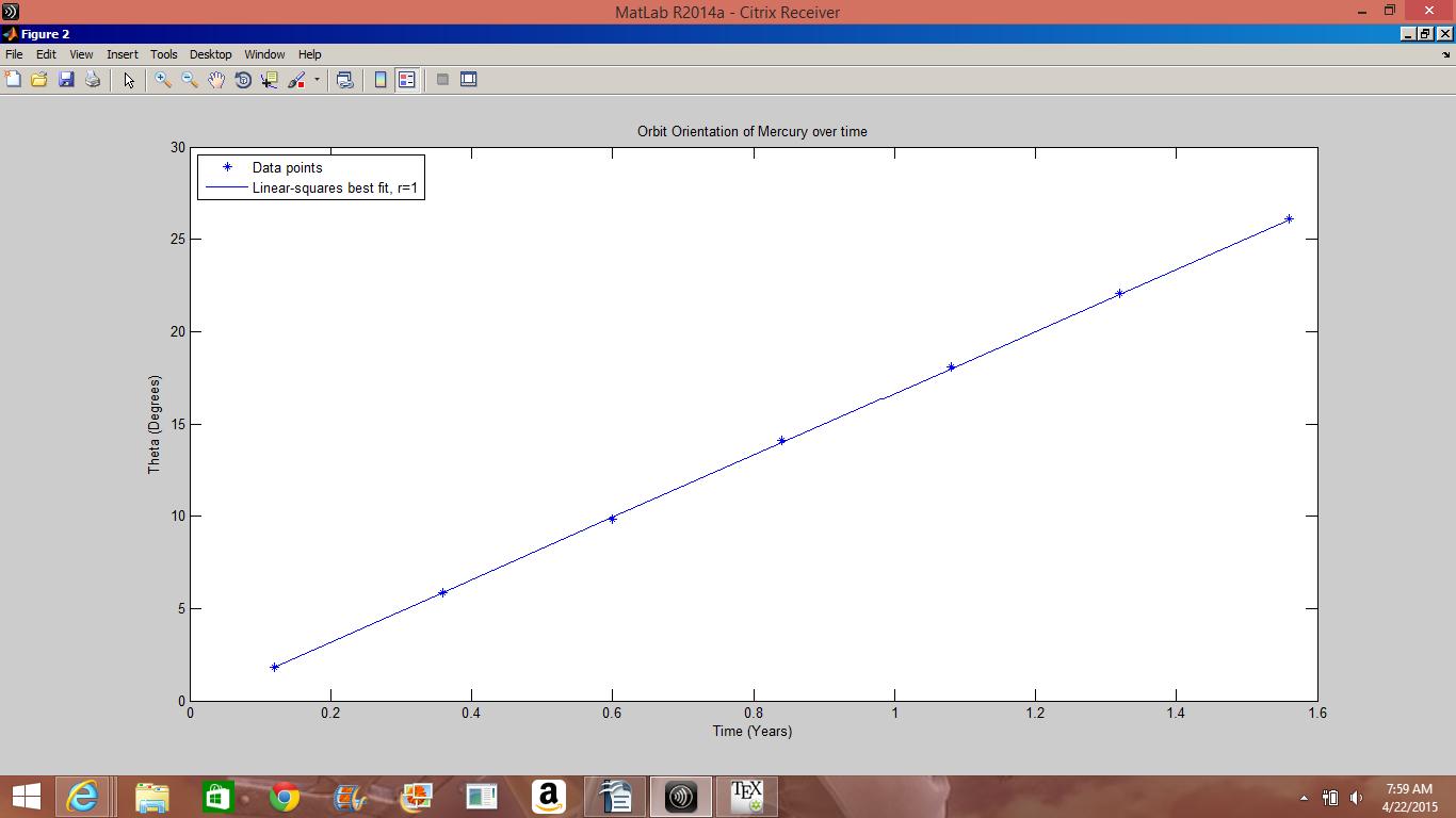
The slope of this graph (C) was calculated to be ; which is close to the true value, . This yielded a precession rate of , as compared to Mercury’s true value, . This corresponds to a percent error deviation of about 10.39.

After completing this extrapolation, I began an investigation into the effect of eccentricity on the precession of the perihelion of a planet’s orbit. I left the both the mass and perihelion values for my test planet to be the same values as for Mercury, however I allowed the semi-major axis length and eccentricity values to vary. 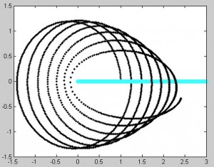Holding the perihelion constant at the value of Mercury’s perihelion results in the expression , where e is the eccentricity and a is the semi-major axis length in astronomical units. Using the same method as given above, I was able to calculate the precession constants C for 7 different Mercurian systems, each with a different value of eccentricity. The results are shown below:

As can be seen by the graph, the best fit for this set of data is a multiple-linear regression fit, of degree 2. Checking this result with Einstein’s expression for the precession rate:

We see that the precession rate is indeed inversely proportional to .

Here is a link to my updated Mercury Precession code:
https://docs.google.com/a/vassar.edu/document/d/1fw8L5ZvhqMMVMYltkJH6Ac425KrmnbbDUJs_6GV7aPI/edit?usp=sharing

And a link to my Mercurian Eccentricity code:
https://docs.google.com/a/vassar.edu/document/d/1eqEBSExnBQZRgFUq9GYQDdjTqC9EODRIR0llXQv7sMw/edit?usp=sharing

References:

Computational Physics by Nicholas J. Giordano and Hisao Nakanishi

Vankov, A.A. “Einstein’s Paper: Explanation of the Perihelion Motion of Mercury from General Relativity Theory”.