
Our larger project goal was to model a three-body system where one object was orbiting a second (larger) one, while an even smaller one was orbiting the first body. The classic example of this system is the earth-moon-sun system.
This second goal was much more difficult than expected considering the relative simplicity involved in reaching the first project goal (simulating the earth’s orbit of the sun). Listed below are some of the different steps that were taken in the direction of this goal. We were not yet successful.
1.
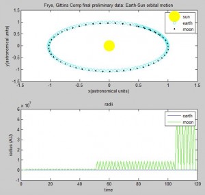
We started out with the entire system: trying to plot the three-body system using the Euler-Cromer method.
And part of it was correct: the earth was orbiting the sun in 1 year. The moon was also orbiting the sun in 1 year. However, the moon was only orbiting the earth 1 time in 1 year, as opposed to about 12 times. Also, according to the program, the radius of the moon was behaving extremely strangely, oscillating sharply between some value for some period of time, then that value would grow a large amount (several orders of magnitude). It would then continue to oscillate.
2.
To confirm the above observation about the moon’s apparent 1 orbit around earth, we changed $dt$ to be extremely small and zoomed in very close to the orbit to examine the moon’s motion more accurately (note the axis in the figure below).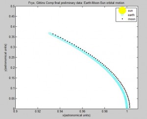
This figure shows that the moon is not orbiting the earth in the correct way.
3.
Our first hypothesis for the incorrect motion was that our initial velocities were incorrect. The image below shows:
Initial velocity of Earth = 2*pi AU/year
Radius of moon’s orbit = 1.0026 AU (the actual distance)
Initial velocity of the Moon = 2.5 AU
Which was one of our attempts at changing the initial velocities of the bodies. Based off the dramatic responses in the simulation upon changes in initial velocity, we assumed that our hypothesis was either entirely or partially correct.
The next step was to play more with the velocities of the bodies. This resulted in somewhat hectic and clearly incorrect figures. This method was not working as we wanted it to.
Taking a step back, we decided to simplify the system into one that we are more familiar with. Having the “Earth” move in a straight line while the moon orbited it would provide a simpler system to study and model. If we could master this simpler system, it would (hopefully) be easy to shift into a circular motion of the earth instead of a linear one.
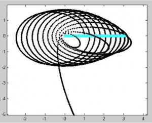
4.
Initial distance between the moon (black) and the earth = 1AU
Linear velocity of earth (blue) = 0.1AU/year
Initial x velocity of the moon = 2.4*pi
dt = 0.01
using
(1) 
(2) 
5.
Initial radius of the moon (black) = 1 AU
Linear velocity of earth (blue) = 0.5 AU/year
Initial x velocity of the moon = 2.2*pi AU/year
dt = 0.005
using
(3) 
(4) 
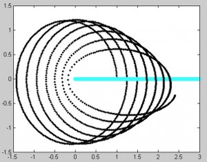
This was becoming a study of how different velocities affect the orbital motion of the two-body system. Unfortunately, the orbit of the moon was not behaving as we wished, even in this simpler program. The orbit began to collapse into itself and the Earth moved too fast for the moon to continue to orbit it. Instead, the moon continued to move in an elliptical motion for some time, but its orbit was completely disconnected from the movement of the moon. Then the orbital motion was lost altogether.
After days of tinkering with the Euler-Cromer method to no avail, we decided to take an even further step back and rethink how to describe the situation of the 3 body system. What might be an easier and more consistent way to describe a circular or elliptical orbit? We decided upon using sine and cosine equations to describe the motion of Earth and the Moon. Although this system brought some of its own problems, mainly programming the system to move, it worked much better than the Euler-Cromer Method and we were able to put all three bodies in the same program. The moon orbit was still slightly unstable, veering off the orbit of the Earth at pi/2 and 3*\pi/2. We determined this was due to the elliptical nature of the orbits, and so specified the major and minor axes of the orbits. This fixed the issue. The problem of actually seeing a body move continues to be a problem, however, as the orbits just look like spinning ovals at the moment. As we continue to work on the program, hopefully we will find a way to represent just a body moving in space with perhaps a thin line to represent the orbit.
All Matlab Codes are listed chronologically (relative to the order in this post) in this Google Doc:
https://docs.google.com/document/d/1-pW6mJHuNV96lPBclSJBbOHwxXdHfXjnpb3cJLJO-30/edit?usp=sharing
It is not the most convenient way to view the codes, but they are color coded to make them easier to look at separately. This was the most convenient way to organize them considering there are so many.
New Resources
- Williams, Dr. David R. “Earth Fact Sheet.” Earth Fact Sheet. NASA, 01 July 2013. Web. 22 Apr. 2015.
- Williams, David R. “Moon Fact Sheet.” Moon Fact Sheet. NASA, 25 Apr. 2014. Web. 22 Apr. 2015.
- “Introductory Astronomy: Ellipses.” Introductory Astronomy: Ellipses. Washington State University, n.d. Web. 22 Apr. 2015.
- “MATLAB Graphics 2D.” Ku Leuven. Katholieke Universiteit Leuven, n.d. Web. 22 Apr. 2015.
- Meshram, Ashish. “3D Visualization of SUN, EARTH and Moon.” MATLAB Central. N.p., 16 July 2013. Web. 22 Apr. 2015.

It would be helpful if you numbered your figures. In your 2nd figure, do you mean the radius of the Moon or the radius of the Moon’s orbit about the Earth?
Sensibly, you resorted to an analytical method when your computational method did not make sense. That gives you a good sense on how to expand your computational method to a 3-body system. This is a good place to investigate the limits of your computational method? Would the Runge-Kutta method have any advantages here over the Euler-Cromer method?