However entertaining modeling a drunk student back home after a long night may be, there is a physical system that corresponds to this movement. For example, gases and liquids both move according to Brownian motion. Brownian motion is the movement where molecules are free to move throughout their container. This movement is both based on random movements and on collisions with other molecules within the container. When looking at one molecule of gas or liquid, this movement appears completely random.

Although my programs model the motion of a wasted student, this random motion can be compared to Brownian motion easily. Not only that, but I can add additional and real physical variables to the code. I decided to focus mainly on drift. Drift for a drunk student can be thought of as a sober and conscious step towards their destination in addition to the random chance of stepping in that direction. This results in biased random motion, or random motion that is directed towards a specific region. In the college student’s case, it could be towards their room or a bathroom. Most Brownian motions in real physical systems include drift. Drift of gas can be caused by a temperature gradient, pressure gradient, physical force, or electromagnetic force.

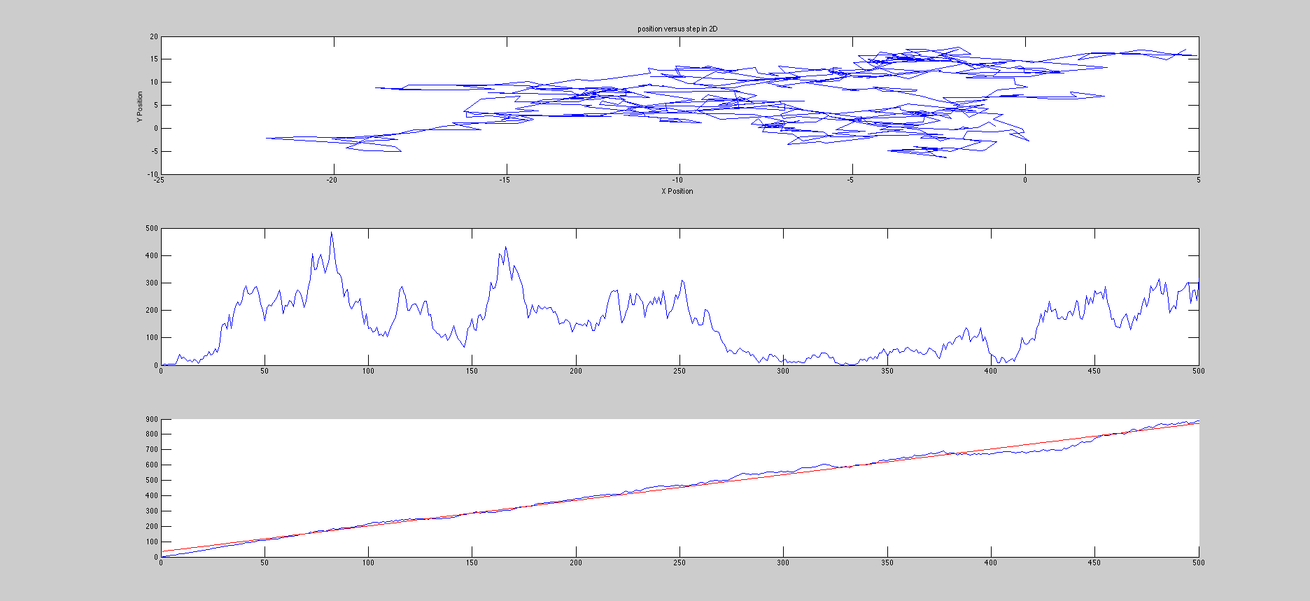
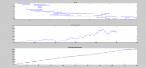
My Matlab codes were designed to plot and determine the displacement squared of 3 different types of “walks.” The first is a very basic random walk. In this system, the walker has an equal chance of taking a step in the positive and negative x and y directions (Figure 1). This can be seen as a simplified system with completely homogenous conditions and one single molecule. The next system is a slightly more realistic system with more complicated and random directions (Figure 3). This is a better approximation for Brownian motion since it allows for the particle to move in any direction with a variable distance traveled for each time step. This also simplifies the system down to homogenous conditions. My final code is a manipulation on the first to account for drift (Figure 5).

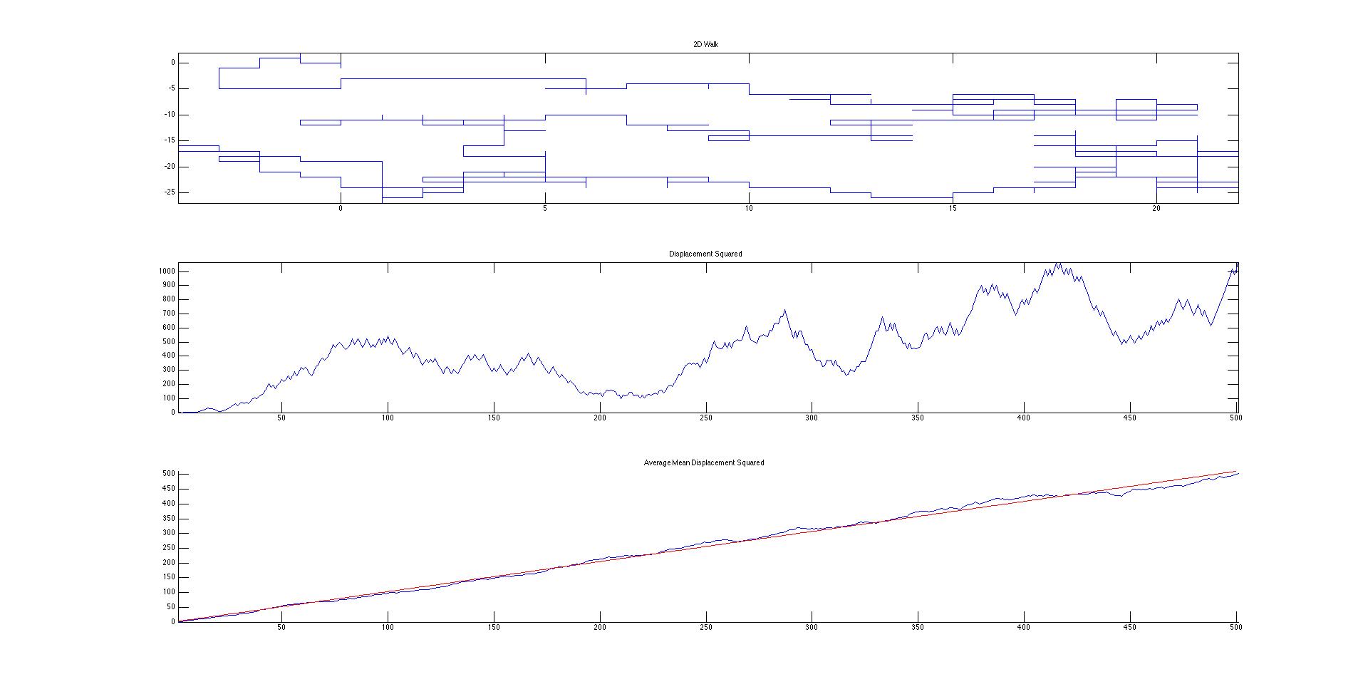
Figure 1. Drunken Motion in 2D. No variables.

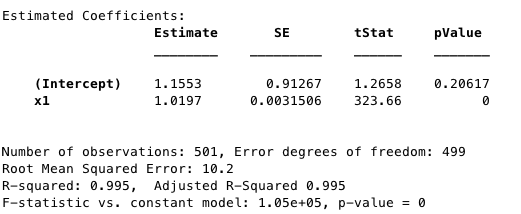
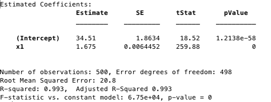
Figure 2. Statistics of Figure 1. Calculated with fitlm function of MATLAB.

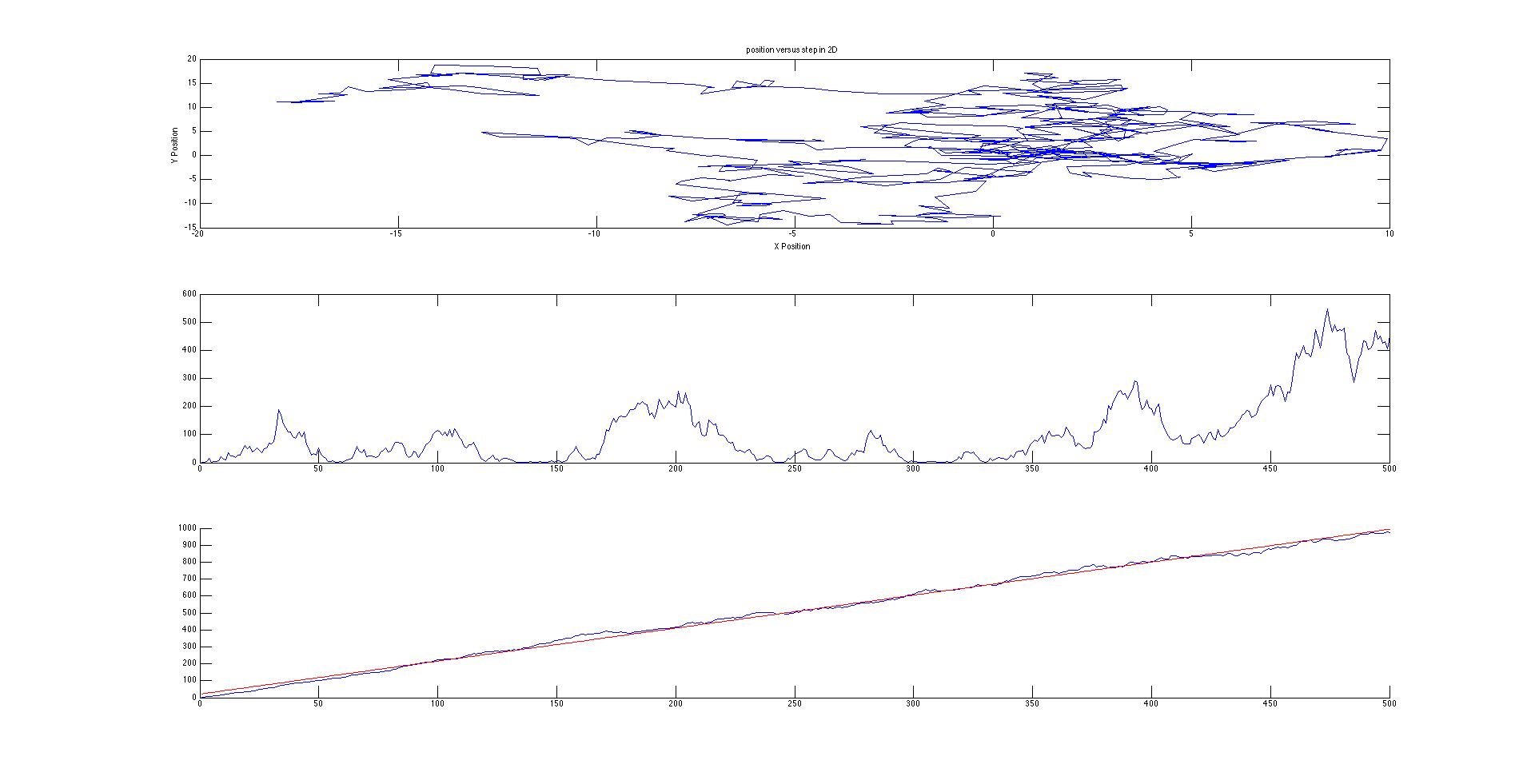
Figure 3. Brownian Motion in 2D

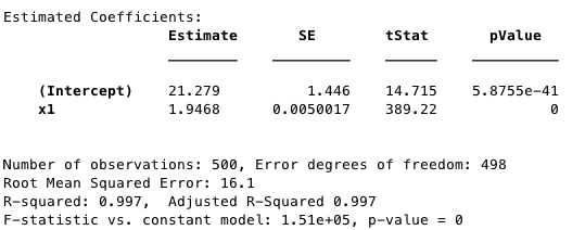
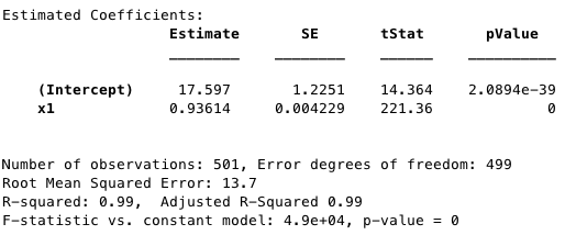
Figure 4. Statistics of Figure 3. Calculated with fitlm function of MATLAB.

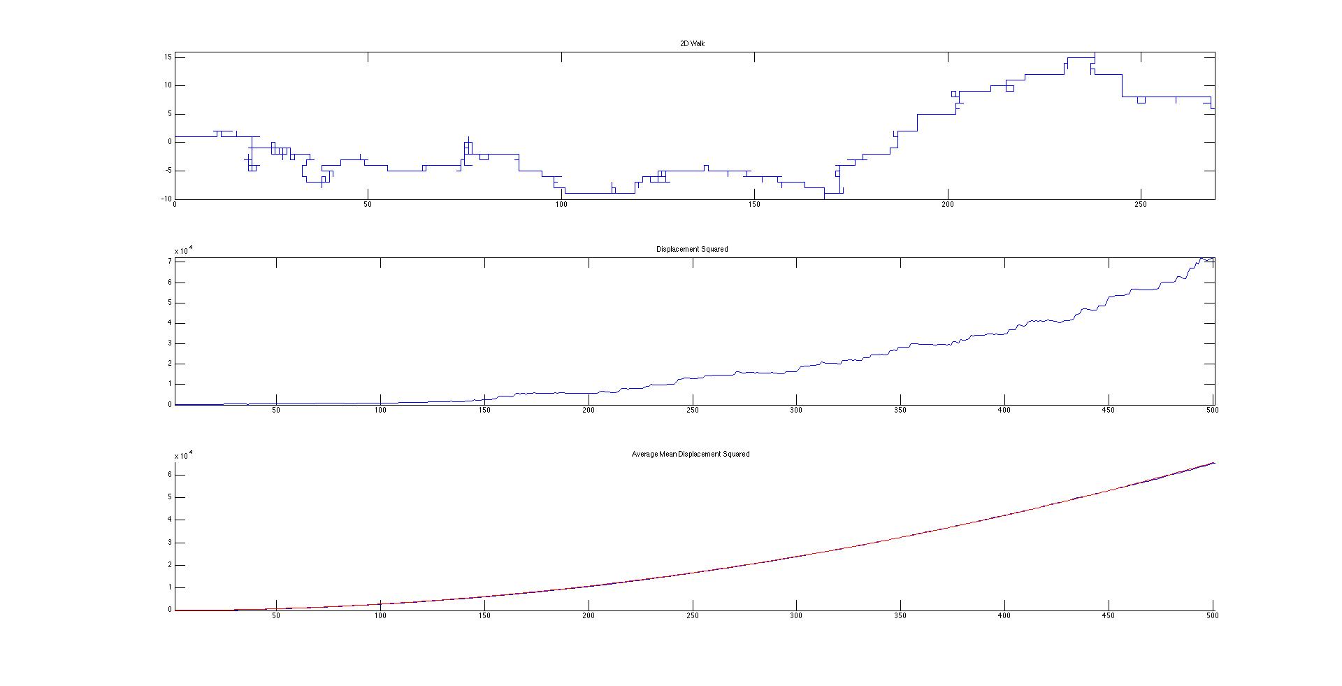
Figure 5. Drunken Walk with drift assigned with a 10% chance of taking 5 steps in +x or +y direction. fit=0.2550t^2+1.0161t+68.1101. R-squared=1.0000

Not only is drift visible on the motion map, the mean displacement squared is magnitudes larger between Figures 1 and 5. When drift was added, a second diffusion constant had to be added since the equation for mean displacement squared became parabolic. Since I am not comparing the mean squared displacements to a system with density (there is only one particle in my system), I can simplify the diffusion constants to be the slopes of their respective best fit lines. According to Figures 2,4, and 5, the diffusion constants are very precise and accurate (error is much less than 1% for linear diffusion), which indicate a statistically significant difference between the different walk methods.

The difference drift makes is considerable. This is important to keep in mind when considering chemical, biological, and physical systems. For example, a higher amount of drift, caused by a higher temperature or lower density on one side of a semi permeable membrane, alters solvent flux. Future directions for my experiment would be comparing the different sources of drift to each other. I would be very interested in modeling the real movement of solutes across a membrane under different gradients, such as temperature or solute density.

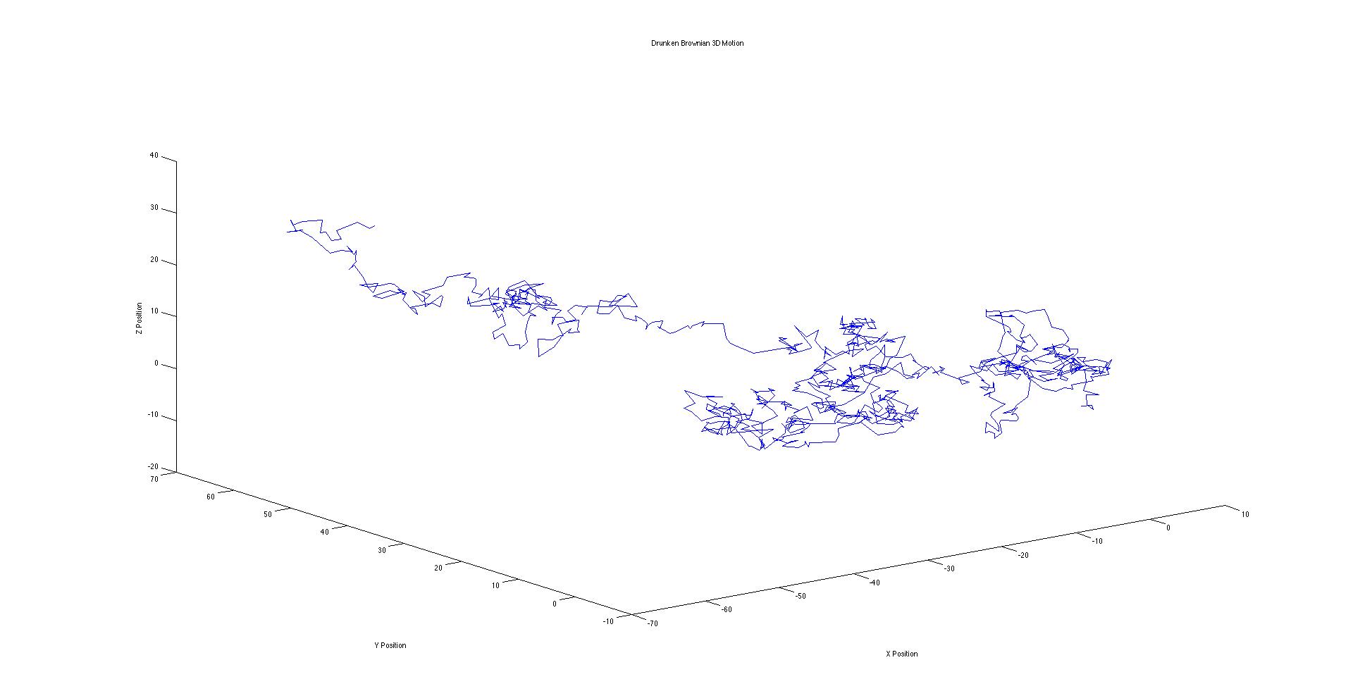
Figure 6. Brownian Motion in 3D. This isn’t all too significant to the rest of my project, but it is a visual representation of the path a liquid or gas molecule takes in a 3D homogenous box.

All 4 of my codes can be found here-https://docs.google.com/document/d/1nvyB5giUicIIiCJuKNKTwJagBlepP8J-IOQsMeMgB7Q/edit

https://docs.google.com/a/vassar.edu/document/d/1nvyB5giUicIIiCJuKNKTwJagBlepP8J-IOQsMeMgB7Q/edit

Brownian Motion of a Drunkard

Random Unit Vector 2D Motion of a Drunkard

As shown by the standard error of the slope within slopes of the displacement squared, the Brownian Motion has a statistically significant larger displacement squared. This is before I alter the 2D code to account for more drunken chance variables. This will serve as a good baseline to see how the mean displacement changes after each variable is added or combinations of variables are tested. I chose to use brownian motion as the standard since it is purely random in every way (in my code). The direction of a step and length are always randomized. I am very pleased with how my codes came out and the visualizations they provide. I apologize for the poor quality of screenshots but they will not look this way in the final project. The top subplot is one representation of the random movement. The second is a displacement squared of one walk. The final in blue is the mean of all of the displacement squareds. The red is the best fit line with the statistics below.

This will serve as my jumping off point to compare Brownian motion of a drunkard (a gas) to a college student on the weekend with several variables and options besides just taking steps. I am curious to see how much I can alter the mean displacement squared with various variables and different weights. Unfortunately, I still need to collect more data outside of class to correctly weight the variables. I’m still catching up on other work from tech week.

I have a preliminary code for the two dimensional random walk. I think it would be much simpler for me to use a displacement needed to get to a location instead of making it to a location for now. I do not have the data displayed on the figure but it is in the matrices. I also have a preliminary code for Brownian Motion but it is very similar to 2D motion. The largest difference is that it does not follow unit vectors. I would like to see how this could affect displacement. I still need more time to finish up my fits and correct for proper units within those fits but I should be in pretty good shape. I would also like to tinker more with the Brownian Motion code to come up with more interesting visualizations. Comparing pure Brownian motion with my novel 2D walk code is my ideal case. Adding more variables to my 2D walk code will come later since I would still like to compare the differences between random 2D walk and Brownian motion. In order to add more variables, I only need to add more “elseif”‘s to my program.

Here are my preliminary programs:

https://docs.google.com/a/vassar.edu/document/d/1nvyB5giUicIIiCJuKNKTwJagBlepP8J-IOQsMeMgB7Q/edit?usp=sharing

Through random system analysis, I would like to determine both a trend for 2D motion between 2 locations and how altering specific real world variables can change this trend. I will be using Chapter 7 of the class text the most for the basic bulk of the code. However, I will be developing novel aspects for my code in order to simulate certain variables within the random journey.

This epic journey will be through the weary eyes of a Vassar student struggling and stumbling (strumbling, if you will) their way back from a long and alcohol filled night. We find this student past inebriation and past wasted: at this point, the poor soul is taking random steps in random 90 degree turns back to their room. They even fall down from time to time. However, there is hope yet! They have a friend with them that will guide them back to their dorm with a gentle push from time to time. How long will it take them to make it back?

The random variables listed above (and I will probably find some more) will be simulated by additional conditions in the MATLAB code and represent real and mathematic aspects of random motion. I will analyze their effects and relative weights of each via multiple graphs that will attempt to find a trend or average number of steps for a certain distance. I would then like to increase the distance gradually in order to find an expression for displacement traveled and the number of steps required.

I would like to present my data as scatterplots of steps required. By adding additional variables during the walk, I can compare their individual effects. In addition, I can watch the effects the relative weights each variable has on the outcome. For example, does a higher rate of falling down change the outcome more than less drift induced from the friend? Toying with relative weights can also make the journey more realistic.

This project allows me to use statistical analysis and probability to map the path of an independent data point with variables imposed on it. This introduces a lot of variance in the data and my largest stumbling block (get it?) will be extracting concrete data from this. Data might also be difficult to extract with pure random motion at long distances. This project also leaves different relationships between variables wide open so I can qualitatively compare variables if concrete data is weak.

Week 1

Writing the bulk of the code and determining whether there is a trend without drift.

Week 2

Implementing additional variables and watching their affect on steps required

Week 3

Data compilation and figure creation

Week 4

Hopefully I’m done around here but if not, I might add another variable to the mix and see how it affects the steps required to reach the destination. Data compilation might spill over into this week too.

Dillon Guynup

Computational Physics

I would like to explore a very important question at our college: will I make it back to campus if I am taking steps in random directions this weekend? Starting from the Town Houses, what is the probability of making it back to my room while quite inebriated? In 2 dimensions, this is nigh guaranteed but how many steps will it take? By manipulating the distance traveled, I can find a trend in the average number of steps the student takes and fit a trend line to it.

Not only can this be mapped in MATLAB, I can also insert extra variables into the program. For example, I can introduce non-random movement at random times. In the real world, this could be seen either as a moment of clarity in a drunken mind or a helpful friend pushing you in the right direction. I would like to derive the expression to calculate the number of steps to go back to campus computationally. This could be an example of random drift and could be used to see how drift affects the time it takes to go home. I can add a lot more to this project by utilizing even more variables. For example, what if the student slips? I could add another random chance of a non-random movement this way.

Dillon Guynup

I would like to explore a very important question at our college: will I make it back to campus if I am taking steps in random directions this weekend? Starting from the Town Houses, what is the probability of making it back to my room while quite inebriated? In 2 dimensions, this is nigh guaranteed but how many steps will it take? By manipulating the distance traveled, I can find a trend in the average number of steps the student takes and fit a trend line to it. This should allow me to derive the expression for random movement.

Not only can this be mapped in MATLAB, I can also insert extra variables into the program. For example, I can introduce non-random movement at random times. In the real world, this could be seen either as a moment of clarity in a drunken mind or a helpful friend pushing you in the right direction. I would like to derive the expression to calculate the number of steps to go back to campus computationally. This could be an example of random drift and could be used to see how drift affects the time it takes to go home. I can add a lot more to this project by utilizing even more variables. For example, what if the student slips? I could add another random chance of a non-random movement this way. That’s about it, folks.