Author Archives: sagittins

Earth, Moon and Sun Orbits – Project Discussion and Conclusion

Project Discussion

Our goal for this project was to first model a two-body orbital system such as the Earth orbiting around the Sun using the Euler-Cromer method. The second goal was to model a three-body orbital system, such as the Moon orbiting the Earth while the Earth orbits the Sun.

We were successful in modeling a two-body system, and did quite a bit of work on studying the two- and three-body orbital systems. We tried both a computational approach and a numerical method to different ends. Ultimately, we determined that although the Euler-Cromer Method works is a good way to approach a two-body system, we were unsuccessful in modeling the three-body system using the Euler-Cromer Method.

First, it must be acknowledged that mass is never involved in the computational method. Honestly, we are not sure why, and that might genuinely be the source of the problem. The analytical method we used did need the masses and the sizes, and it worked much better, which raises questions about the computational method that we employed. If we were to incorporate mass into the computational method, however, we may have run into the issue that the sun is significantly more massive than the Earth. Had we attempted to base the movement of the Moon with an equation related to mass, the Moon likely would have jumped orbit from the Earth and gone to orbit the Sun.

Secondly, we would like to bring reference frames into the discussion. We did our project in the reference frame of the sun, but what would have changed if we were approaching the project from the reference frame of the universe? Or the earth? Or even the moon? — Because we approached it from the reference frame of the sun, any effect the earth and moon’s masses had on it would not appear in the simulation. We assumed that this is an acceptable assumption, because the relative masses would make it so that the effect of these two masses would negligibly affect the sun’s motion, but we are not sure if changing the reference frame would change the results.

The conservation of energy law requires the total energy of a closed system to remain constant. In an orbital system, if energy is positive or not conserved, the orbit can turn into a hyperbolic one instead of an elliptical.

In checking the energy of the systems: we first used the equation

(1)   \begin{equation*} E_{E}=-\frac{GM_{S}m_{E}}{2R} \end{equation*}

(2)   \begin{equation*} E_{M}=-\frac{Gm_{E}}{2} \left(\frac{M_{S}}{R} + \frac{m_{M}}{r}} \right) \end{equation*}

Which comes from combining the orbital potential energy and orbital kinetic energy:

(3)   \begin{equation*} E = K + U \end{equation*}

But on second thought, $r<<R$ (where $r$ is the distance between the moon and the Earth, and $R$ is the distance between the Earth and the Sun). So we rewrote the energy of the moon as

(4)   \begin{equation*} E_{M}=-\frac{Gm_{M}}{2} \left(\frac{M_{S}}{R} + \frac{m_{E}}{r} \right) \end{equation*}

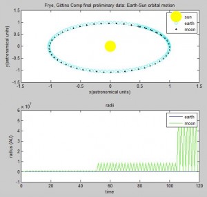
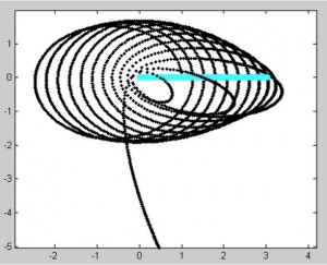
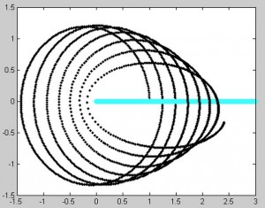
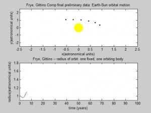
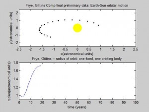
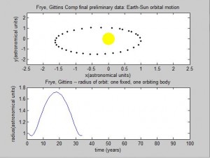
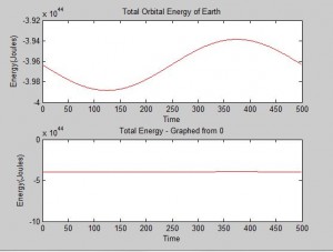
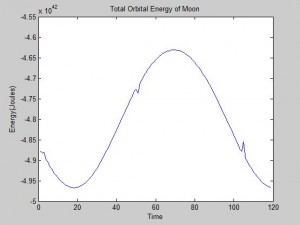
But strange “spikes” appeared in the energy plot, occurring where the radius changes dramatically. The energy plot is sinusoidal, completing one period in one orbit of the earth around the sun. We are not sure why this is so, but at second glance, the amplitude of the sine wave is very very small — it is between 4*10^44 and 4.5*10^44 Joules, so if we plot the energy from 0 the fluctuation is not visible.

Plot of Earths orbital energy for comparison:

Energy

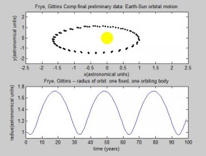
Plot of Moon’s orbital energy:

radiusEnergyofMoon

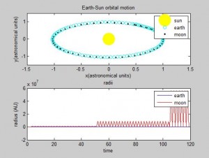
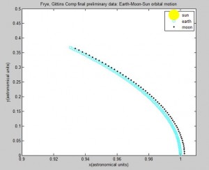
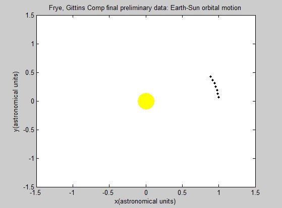
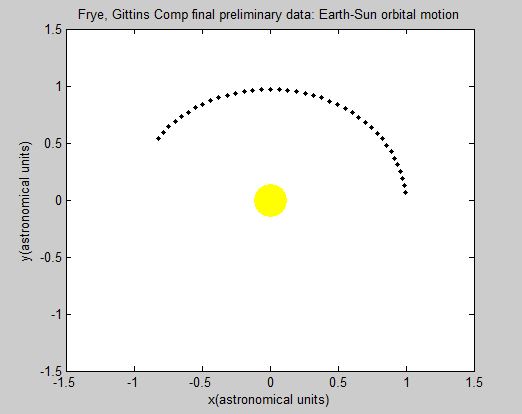
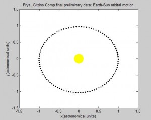
This all raises the question: is the Euler-Cromer method inherently not useful for this problem? There is a good chance the program we wrote was the reason the simulation was unsuccessful. But what other reasons could there be for the program not to work? The Euler-Cromer is an iterative method, which makes a prediction on the next location based on the most recent information. It did work well for the two body system, producing a clean simulation of the Earth orbiting the Sun, which you can see below. (The simpler Euler method is not as viable of a method because over time the calculated information would get further and further from the “true” values, because it does not use the most recent information.)

So why is analytical easier, or at least more effective, in this case? The analytical is more specific than the computational method, because the motion of the system is already known and therefore the method can be tailored for the system. We as programmers are familiar with how and why the Euler-Cromer method works, and we are confident that this method is the best for our physical system. In the same manner, we are confident that our problem lies in how we are updating the x and y position of our orbiting bodies.


gif_4


Link to analytical code:

https://docs.google.com/document/d/1mKmL4spylb1h6PttlyTBY9vIuZmfnLVQhfAzvSX2qBA/edit?usp=sharing

Link to Energy codes:

https://docs.google.com/a/vassar.edu/document/d/1KzZduXpxZ6-_gEja875FwCyn0Yvc_yO69JxQJSsasvA/edit?usp=sharing

https://docs.google.com/a/vassar.edu/document/d/15wfmgWwkx_TbmMf4Untcb5DXdADvH7mSrB8Vs2DKY4Q/edit?usp=sharing

Share

Frye and Gittins – 3 Body System – Sun, Earth, Moon

Our larger project goal was to  model a three-body system where one object was orbiting a second (larger) one, while an even smaller one was orbiting the first body. The classic example of this system is the earth-moon-sun system.

This second goal was much more difficult than expected considering the relative simplicity involved in reaching the first project goal (simulating the earth’s orbit of the sun). Listed below are some of the different steps that were taken in the direction of this goal. We were not yet successful.

1.

We started out with the entire system: trying to plot the three-body system using the Euler-Cromer method.

gif_1


And part of it was correct: the earth was orbiting the sun in 1 year. The moon was also orbiting the sun in 1 year. However, the moon was only orbiting the earth 1 time in 1 year, as opposed to about 12 times. Also, according to the program, the radius of the moon was behaving extremely strangely, oscillating sharply between some value for some period of time, then that value would grow a large amount (several orders of magnitude). It would then continue to oscillate.

Incorrect_moon_1

2.

To confirm the above observation about the moon’s apparent 1 orbit around earth, we changed $dt$ to be extremely small and zoomed in very close to the orbit to examine the moon’s motion more accurately (note the axis in the figure below).Incorrect_moon_2

This figure shows that the moon is not orbiting the earth in the correct way.


3.

Our first hypothesis for the incorrect motion was that our initial velocities were incorrect. The image below shows:

Initial velocity of Earth = 2*pi AU/year

Radius of moon’s orbit = 1.0026 AU  (the actual distance)

Initial velocity of the Moon = 2.5 AU

Which was one of our attempts at changing the initial velocities of the bodies. Based off the dramatic responses in the simulation upon changes in initial velocity, we assumed that our hypothesis was either entirely or partially correct.

The next step was to play more with the velocities of the bodies. This resulted in somewhat hectic and clearly incorrect figures. This method was not working as we wanted it to.

gif_2

Taking a step back, we decided to simplify the system into one that we are more familiar with. Having the “Earth” move in a straight line while the moon orbited it would provide a simpler system to study and model. If we could master this simpler system, it would (hopefully) be easy to shift into a circular motion of the earth instead of a linear one.


4.

Initial distance between the moon (black) and the earth = 1AU

Linear velocity of earth (blue) = 0.1AU/year

Initial x velocity of the moon = 2.4*pi

dt = 0.01

using

(1)   \begin{equation*} \ x_{M}new = x_{M}+v(x)_{M}new*dt \end{equation*}

(2)   \begin{equation*} \ y_{M}new = -2*xnew*dt + y_{M} + v(y)_{M}new*dt \end{equation*}

Incorrect_moon_3

5.

Initial radius of the moon (black) = 1 AU

Linear velocity of earth (blue) = 0.5 AU/year

Initial x velocity of the moon = 2.2*pi AU/year

dt = 0.005

using

(3)   \begin{equation*} \x_{M}new = x_{M}+v(x)_{M}new*dt \end{equation*}

(4)   \begin{equation*} \y_{M}new = -2*xnew*dt + y_{M} + v(y)_{M}new*dt \end{equation*}


Incorrect_moon_4

This was becoming a study of how different velocities affect the orbital motion of the two-body system. Unfortunately, the orbit of the moon was not behaving as we wished, even in this simpler program. The orbit began to collapse into itself and the Earth moved too fast for the moon to continue to orbit it. Instead, the moon continued to move in an elliptical motion for some time, but its orbit was completely disconnected from the movement of the moon. Then the orbital motion was lost altogether.


After days of tinkering with the Euler-Cromer method to no avail, we decided to take an even further step back and rethink how to describe the situation of the 3 body system. What might be an easier and more consistent way to describe a circular or elliptical orbit? We decided upon using sine and cosine equations to describe the motion of Earth and the Moon. Although this system brought some of its own problems, mainly programming the system to move, it worked much better than the Euler-Cromer Method and we were able to put all three bodies in the same program. The moon orbit was still slightly unstable, veering off the orbit of the Earth at pi/2 and 3*\pi/2. We determined this was due to the elliptical nature of the orbits, and so specified the major and minor axes of the orbits. This fixed the issue. The problem of actually seeing a body move continues to be a problem, however, as the orbits just look like spinning ovals at the moment. As we continue to work on the program, hopefully we will find a way to represent just a body moving in space with perhaps a thin line to represent the orbit.

gif_3


All Matlab Codes are listed chronologically (relative to the order in this post) in this Google Doc:

https://docs.google.com/document/d/1-pW6mJHuNV96lPBclSJBbOHwxXdHfXjnpb3cJLJO-30/edit?usp=sharing

It is not the most convenient way to view the codes, but they are color coded to make them easier to look at separately. This was the most convenient way to organize them considering there are so many.

New Resources

  1. Williams, Dr. David R. “Earth Fact Sheet.” Earth Fact Sheet. NASA, 01 July 2013. Web. 22 Apr. 2015.
  2. Williams, David R. “Moon Fact Sheet.” Moon Fact Sheet. NASA, 25 Apr. 2014. Web. 22 Apr. 2015.
  3. “Introductory Astronomy: Ellipses.” Introductory Astronomy: Ellipses. Washington State University, n.d. Web. 22 Apr. 2015.
  4. “MATLAB Graphics 2D.” Ku Leuven. Katholieke Universiteit Leuven, n.d. Web. 22 Apr. 2015.
  5. Meshram, Ashish. “3D Visualization of SUN, EARTH and Moon.” MATLAB Central. N.p., 16 July 2013. Web. 22 Apr. 2015.
Share

Gittins & Frye – Preliminary Data

The first simulation we wrote was a simulation for the orbital movement of a planet such as Earth as it orbits the Sun. The orbital motion program was built using the Euler-Cromer method, as specified in the earlier blog post, with new “guesses” for position iterating through a loop for a specified number of calculations.

Although this program is great for visualizing the orbital motion of an object, there were many assumptions made in the creation of the simulation.

The most blatant simplification made was that this is a two-body system. There are of course many more planets in the real solar system, but for the sake of this first simulation, they were ignored. It is not a study of their true motion, but more a simplified circular orbit of a planet (Earth) about the sun. The mass of the Sun and Earth are not even part of the program because they are not significant factors when the mass of the Sun is significantly larger than the mass of the Earth.

We assumed that the sun does not move. Although this is almost true (because Ms>>Me), in reality, the Sun would move in a small orbit that responded to the Earth’s larger motion. Additionally, the Earth would not move in a perfect circular motion but rather in an elliptical direction.

However, this visualization remains a valuable tool for both the conceptualization of an orbital system and also for the further understanding of the Euler-Cromer method. Because it is iterative, and uses the most recent information to continue its guesses, making the approximation relatively accurate.

This is a useful program, but can definitely be more specific and more physically accurate. Our next step should be to try to either add a second planet, or for an extra challenge, adding the moon orbiting our already-orbiting Earth. Additionally, there should be a way for matlab to generate a more visually pleasing result, with a moving planet that leaves a tail behind for us to see the final orbit.

Screenshots of the orbital movement:


EarthSunRevised_1 revised 2     revised3


We then explored the affect on the orbit if the initial velocity was higher than our original initial velocity. We discovered that by increasing the initial velocity by 10%, the orbit would become elliptical, with the Sun at an off-center focus point. The radius is 1AU at the perihelion, or the fastest moving point, and approximately 1.72 at the aphelion. This is consistent Kepler’s First Law.

velocities1velocities2velocities 3velocities4

The Matlab script:

https://docs.google.com/a/vassar.edu/document/d/1gHvpNnY2pMAh-y2DEihLfF9S7EOxLUb2zZ_FVGl99Qo/edit?usp=sharing


Share

Orbital Motion Simulation – Frye and Gittins


We plan on modeling objects in orbital motion, namely the sun and earth, the earth and moon, the three together, and finally an orbit of two large-massed bodies, such as the sun and another star.

The programming steps we need to take are straightforward in theory. We have already settled on using the Euler-Cromer method on MatLab to simulate the motion. We have access and prior knowledge of Newton’s laws and Kepler’s laws of motion, as shown below.  The potentially difficult part will be writing a program that will be able to track the motion of several bodies simultaneously, with the capability of visualization, such as a moving graphic.


(1)   \begin{equation*} \ F_{G}=\frac{GM_{S}M_{E}}{r^{^{2}}} \end{equation*}


where Ms is the mass of the sun and Me is the mass of the earth.


Kepler’s Laws:

  • All planets move in elliptical orbits with the Sun at one focus.
  • The line joining a planet to the Sun sweeps out equal areas in equal times.
  • If T is the period and a the semimajor axis of the orbit, then T^2/a^3

(2)   \begin{equation*} \frac {d^{2}x}{dt^{2}} = \frac {F_{Gx}}{M_{E}} \end{equation*}

(3)   \begin{equation*} \frac {d^{2}y}{dt^{2}} = \frac {F_{Gy}}{M_{E}} \end{equation*}


from which we can derive the equation:

(4)   \begin{equation*} \ F_{Gx}=-\frac{GM_{S}M_{E}}{r^{2}}\cos{\theta}=-\frac{GM_{S}M_{E}x}{r^{3}} \end{equation*}

for the x-direction. A similar equation can be found for the y-direction. For the equations of motion that will be put into the Euler-Cromer program, we will use equations similar to those derived in Giordano.


(5)   \begin{equation*} \ v_{x,i+1}=v_{x,i}- \frac{4\pi^{2}x_{i}}{r_{i}^{3}}\Delta{t} \end{equation*}

(6)   \begin{equation*} \ x_{i+1}=x_{i}+v_{x,i+1}\Delta{t} \end{equation*}

(7)   \begin{equation*} \ v_{y,i+1}=v_{y,i}- \frac{4\pi^{2}y_{i}}{r_{i}^{3}}\Delta{t} \end{equation*}

(8)   \begin{equation*} \ y_{i+1}=y_{i}+v_{y,i+1}\Delta{t} \end{equation*}


For preliminary data, we hope to have a primitive program that has the capability of simulating a simple Earth-Sun orbit, assuming that the Sun is so massive (compared to Earth) that it does not move. We hope to have an appropriate visualisation, a moving plot, to apply to the data. At this time we will need to heavily research the physics of the situation, including providing details of what is physically incorrect about our simulation and the amount of error these details create. The defense of this simulation, including pros and cons of the Euler-Cromer method in this case, will be in the preliminary data.

The second goal is to make the system more complicated, either adding the moon or another planet to the existing system. As in the first set of data, we will need to analyze it for flaws. We anticipate this to be the most difficult programming challenge, as there are three systems moving simultaneously, and also the most complex error analysis.

Screen Shot 2015-04-01 at 12.10.11 AM

Finally, we plan to model a system in which each mass is in motion, for example, two large suns or a star and a large planet.  At this point, we will be fairly comfortable with the Euler-Cromer method applied to this system. Here, we will truly analyze the flaws with the method and compare and contrast these flaws, and its strengths, with other methods we have learned in class. This will also provide insight into our previous simulations and their errors, as the sun is not un-moving as we assume previously.

two massiv

We hope the final program will appear similar to the ones shown in Giordano and the exploration of orbits done by Moler.


Timeline:

Week 1: Research more equations and pseudo codes that relate to our simulation.

Week 2: Write a primitive program to simulate the earth and the sun orbit. Calculate error.

Week 3: Finish Earth-Sun simulation. Begin writing program for Moon-Earth-Sun by working with program from Week 2. Begin writing primitive program for two massive planets or stars.

Week 4: Finish program for two massive planets or stars. Calculate error. Troubleshoot Moon-Earth-Sun program.

Week 5: Finish all programs and prepare for presentations.


Resources

  1. Giordano. Computational Physics, 2006.
  2. Moler, Cleve. “Orbits,” MathWorks Inc, 2011.
Share

Sarah Gittins and Lily Frye – Orbital Mechanics

Using the Euler cromer method, we will investigate the movement of solar entities in orbit. First, we will write a program that numerically finds the position and velocity of the earth as it orbits the sun. Second, we will write a program that numerically finds position and velocity of the moon as it orbits the earth as the earth orbits the sun. Third, we will write a program that numerically finds the position and velocity of a large star such as the sun as a massive planet orbits it, or rather as they orbit and affect each other. To calculate these movements we will use basic equations of motion and Kepler’s laws.


Screen Shot 2015-04-01 at 12.10.11 AM


Share