The goal for our project was to develop an understanding of how physics methods can be used in the field of financial modeling. Primarily concerned with predicting prices and market shares over time, financial analysts have historically made liberal use of traditional physics and math techniques to best solve different sorts of systems.

A brief literature search indicated that one of the most commonly used physics tools in finance is the Monte Carlo method. Originally developed as part of the Manhattan Project to simulate the penetration of neutrons into a nucleus, the Monte Carlo method has come to refer to the general concept of using a massive amount of randomly generated numbers to simulate the development of a system based on some sort of probability distribution.

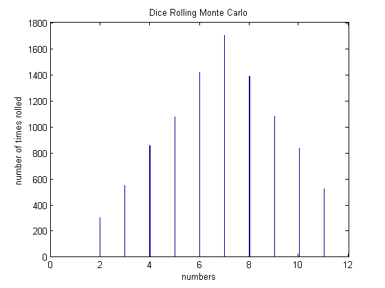
We began the project by familiarizing ourselves with basic Monte Carlo methods. First, we simulated the results of rolling two dice, simply generating two random numbers between 1 and 6 for an arbitrarily large amount of times. This basic method produced a distribution that described the most frequent combination of rolls. As expected, the mode of the distribution was 7. Next, we worked on a slightly more challenging problem, using Monte Carlo methods to numerically integrate a function. We used a rather trivial case, a circle inscribed in a unit square. The program dropped an arbitrarily large amount of points onto the system and counted how many fell within the bounds of the function. The ratio of this count to the overall number of points simulated the area of the function. The value of pi was obtained, confirming that our method was effective.

The next step was to decide which specific financial methods we would explore in depth. We decided to pursue two areas, the calculation of stock option prices and the evolution of the price of a good in a simple market over time.

A stock option is a financial tool used by traders to bet on the price of a stock over time. It allows the said trader, for a certain price, to be able to value the stock at a fixed price no matter how it changes in the overall market. A call option gives the trader the right to buy a stock at a fixed price over time, even when the market price rises significantly. Similarly, a put option gives the right to sell the stock at a fixed price over time, most useful when the stock price drops in the market over time. The problem in question is then to calculate the initial fee for which the trader can buy the right to have one of these options on the stock.

We explored three methods for pricing these options. The first was the Black Scholes method, which relies on knowing the values of several crucial parameters and the cumulative distribution that these parameters define. Equation for Black-Scholes where $C$ is the price of the option:

(1)  

where

(2)  

and

(3)  

$N(d_1)$ is the standard normal distribution of $d_1$ and $N(d_2)$ is the standard normal distribution of $d_2$ where $d_1$ and $d_2$ are a distribution.

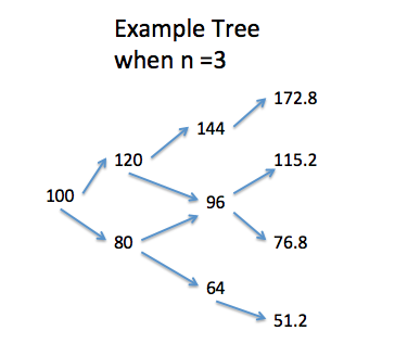
This method proved to be rather rigorous as it necessitated at least basic knowledge of statistical modeling and the exact value of the parameters. The second method, the Monte Carlo distribution of pricing, was more elegant. It used a uniformly distributed set of random numbers between 0 and 1 and plugged the set into an equation that needed only the original price of the stock, the interest rate, and the volatility of the stock. Finally, the most elegant method to calculate the price of an option involved the use of binomial trees. Beginning with a strike price and a theoretical return on the stock, the binomial method calculated the value of the stock at an increasingly large number of nodes in the tree and then plugged these nodes into an equation that would value the price of the option.

The second system we studied was based off the Ising model used to simulate the evolution of a thermodynamic system over time. The most prominent application is the simulation of a ferromagnetic material whose constituent atoms possess spin characteristics that influence their neighbors. These spins naturally tend to align themselves in the same direction, and thus we have started with a ferromagnetic system in which all spins are aligned. We then simulate stochastic changes in the system that occur because of energy added by the temperature in a heat bath. As temperature rises, the greater there is that one of the spins will orient itself in a way that requires adding energy to the system. This is because the extra heat from the increased temperature supplies extra energy. The system is solved using a Monte Carlo method to calculate the probability of each atom flipping its spin per unit time, based on the interactions with its neighbors and the overall energy. The higher the energy, the higher the probability of flipping the atom. The average spin of the system is called the “Magnetization” and is a good way to represent how magnetic the metal is.

This system is then applied to the world of finance by simulating an evolving market of agents who can either choose to buy or sell a good, which is shown by:

(4)  

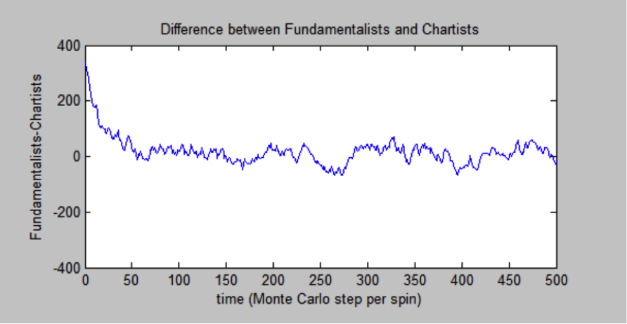
The decision to be a buyer or a seller influences the decisions of the nearest neighbors. However, all agents also are aware of a systematic trend in “magnetization” which in this case represents the price of the good in question. If there are more buyers than sellers, the price will be rising, so buyers will wish to join the sellers group to make a profit off of their good. The Monte Carlo method once again calculates the probability of these agents changing their identities, displaying the trend in price over time. The probability is given by:

(5)  

Then, the probability of an agent remaining/becoming a buyer is given by:

(6)  

(7)  

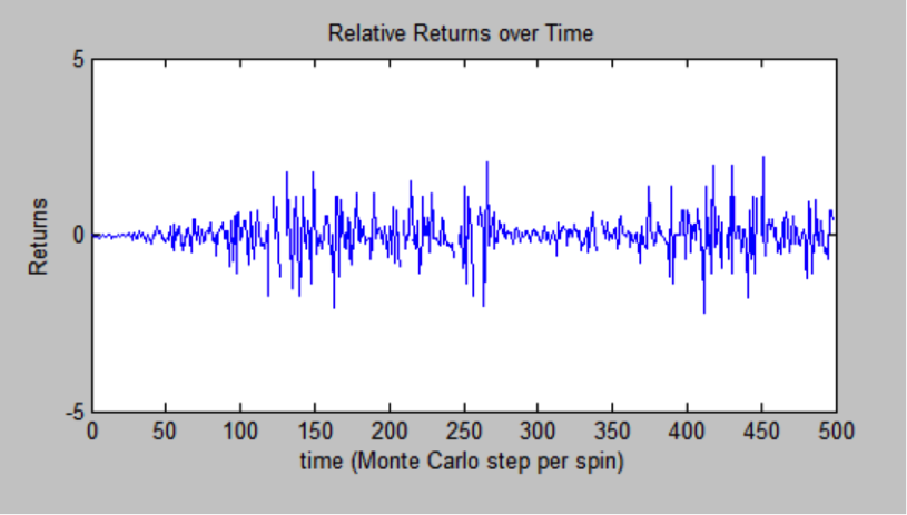
It is possible to see the stochastic nature of the pricing evolution over time, as well as the distribution of buyers and sellers in a market given some initial conditions. As we discovered, when buyers and sellers grouped with agents of their own identity, price is more volatile.

Below is a table that summarizes every method we have used, as well as providing the name of each file, found at this link https://drive.google.com/a/vassar.edu/folderview?id=0B01Mp3IqoCvhflF5azV4bHY2V0c3Vks0VXVyQkIxcnR4RmFaNDhVWEQtZGZSR2t6V2VWOHc&usp=sharing#:

After investigating the call and the put option last week, we decided to continue to investigate option or derivative trading. This time we looked at how to program binomial trees in MatLab. For a quick refresher a call option is when the owner of the asset, which can be a stock or portfolio, has the right to buy the asset at the pre-determined strike price. A put option is when the owner has the right to sell the asset at the pre-determined strike price. This means that if the asset price goes below the strike price, the put option is advantageous and makes the owner money. If the asset price goes above the strike price then the call option becomes the money making option.

So what exactly does a binomial tree look like. Below is the an example of a binomial tree when n=3 which means that past n=0 there are three distinct division. In this case at n=0 the price of the asset is 100 dollars. Binomial trees are interesting because unlike the Black-Scholes method, which was previously discussed in last weeks post, the binomial tree provides the user with a flexible way to price the option. In this example at each node the price of the asset has two alternatives it can either go up in price or down in price. Unlike the Black-Scholes model the binomial tree provides a period to period transparency in the price of the option. It is important to note that this binomial tree does not follow the same definition that a typical discrete mathematics textbook would describe a tree. This is because the binomial option pricing tree contains cycles, where as in a strict mathematically definition trees cannot contain cycles.

 (Each number is the possible price of the asset).

The binomial tree is more advantageous in pricing American options. This is because for an American option the owner at any point can exercise the option before the maturity date (when the option expires). The binomial tree works backwards to find the value of the option at T=0, when time is equal to zero. This helps determine how much one is willing to pay for the option. The binomial tree finds the difference in price between the original asset price, and the price at another discrete time interval, using the function max(K-P,0) , where K is the strike price, and P is the price of the asset at T=0. This function max(K-P,0) is used for a put option, and described more in our code.

It is important to discuss the variables the binomial tree is dependent on. It is dependent on $\sigma$ which is volatility, simply it is just the standard deviation in returns of an asset or portfolio, $r$ is risk neutral interest rate, $u$ and $d$ are percentages the asset either goes up or down at each stage of the tree. The formula for backwards induction to find the original value of the asset is…

(1)  

where $V_u$ is the upper price at a discrete stage, and $V_d$ is the lower price at a discrete stage. A discrete stage meaning n=1,2… We know need to look at what p is, well p simulates the geometric Brownian motion of the underlying stock or asset with parameters $r$ and $\sigma$. p is given by the equation below:

(2)  

We have finished the pricing of an American put option for a binomial tree when n=3. And plan on continuing to work on the code for the option pricing method to work for an arbitrary number for n, and hope to have completed by our next post.

The past week has been spent turning the basic ferromagnetic spin model (isingtest.m) created last week into a model of a basic financial system. In the ferromagnetic model, the spins of constituent atoms were represented by discrete spin values of 1 or -1. In this model, we will use the analogous atoms to represent agents in a market. This market will be based on any arbitrary good or stock, and like the ferromagnetic model, adjacent “agents” will be able to share information and influence each other. Here, the tendency for atoms to align with adjacent atoms represents a tendency of financial agents that work close to each other to use the same ideas.

In this model, a spin value of 1 signifies that an agent is currently buying the good or stock, whereas the value of -1 signifies that the agent is currently selling it. The market is governed by two rules:

1. The first rule is analogous to the ferromagnetic model: adjacent actors influence each other strongly.
2. The second rule introduces an idea analogous to a heat bath. This rule states that the agents in the minority group have a special kind of knowledge, so all agents in the market will want to be part of that minority group.

In order to initialize this market, we create a grid to store whether or not each agent is a buyer or seller. We initially assigned the majority of agents to be buyers, represented as white pixels. The sellers are interspersed as blocks throughout the market, represented by the black pixels. Below is an example of what an initial market might look like:

From here, our monte carlo method cycles through every agent in the market, using its position relative to its neighbors as well as an overall market trend to calculate the “field” that pushes it toward one strategy or another. After every iteration, the display of the grid was altered accordingly. The equation for this field is below:

(3)  

The first term in the expression is analogous to the spin alignments, whereas the second term is representative to the individual agent’s view of the whole market. The value C corresponds to whether an agent will be a “fundamentalist(C=1)” or a “chartist(C=-1).” If the agent is a fundamentalist, it means that he or she will be likely to follow the rule that it is best to try to get into the minority, making the second term negative and pushing it against the first term. If the agent is a “chartist,” it means that he or she is content with being in the majority, and the sign of the second term is the same as the first. Whether or not the agent is a fundamentalist or a chartist is determined by whether or not choosing this strategy will increase the energy, or risk, of the system, which would improve the likelihood of making money. This probability of an agent changing his or her identity is determined with:

(4)  

Then, the probability of an agent remaining/becoming a buyer is given by:

(5)  

(6)  

The second term is the probability that the agent will remain/become a seller. A random number is generated by the monte carlo method and compared to the probability, deciding which strategy the agent in question will use at the current time. Once the code has cycled through every agent in the market, it will update the grid displaying the identity of each agent’s strategy at the given time. The average value of all of the strategies in the market is then taken, as it is representative of the price of the good or the stock. A positive average represents a positive trend in price, because there are more people that want to buy than sell. The opposite is true as well, as a negative average means that there is a surplus of sellers. Taking this average and subtracting from it the average of the last iteration gives use the change in price, or return, created by a shift in the market. An example is displayed below, plotting this average vs. time:

The periods of extreme return in a negative or positive direction correspond to a market configuration where there are large groups of buyers grouped together and large groups of sellers grouped together as shown below:

Conversely, when the returns stay near 0, it is because there is no real trend in the market and it is more turbulent, as such:

Finally, another way to represent this trend is to show the difference between fundamentalists in the market compared with chartists in the market. This difference is displayed below, and it is possible to see that when there is a more extreme difference, there are more extreme changes in the return.

For our final part of this project, we will try to use the autocorrelation function to characterize the volatility of the good over time. We will also try to add another strategy option, as well as possibly exploring a 3 dimensional system. The code for this part is “TwoStrategyMarketModel.m”

Link to Code:

https://drive.google.com/folderview?id=0B01Mp3IqoCvhflF5azV4bHY2V0c3Vks0VXVyQkIxcnR4RmFaNDhVWEQtZGZSR2t6V2VWOHc&usp=sharing

The files are under the name: BinomialTreeNThree.m and TwoMarketStrategyModel.m

The primary goal of this week was to further our understanding of the Monte Carlo method works. To do this we researched basic modes of how the Monte Carlo method operates. The Monte Carlo method relies on the repeated random sampling to obtain numerical results. We decided to demonstrate how this method can be used to illustrate the distribution of numbers of two dice rolled for an arbitrarily number of times. 

As expected, 7 is rolled the most amount of times.

One of the most basic Monte Carlo methods is the calculation of the value of pi. Look at the following picture, in which a black unit circle is inscribed into a white square: 

We know that the ratio of the area of the circle to that of the square is pi/4. If you need to prove this to yourself, simply divide the area of a circle by that of a square whose sides are twice the length of the circle’s radius. Now, imagine that you dropped a series of evenly and randomly distributed darts across the image. If you counted them, the number of darts within the circle should be about pi/4 times the amount of total darts dropped. It is much easier to simply count these darts than to try any other mathematical measurement. The following code allows us to simulate this scenario by randomly selecting coordinates within the image above. If the randomly selected coordinate has a value of 0, it is black and thus it is counted as having landed in the circle. Most of the trials yield a value of about 3.09, relatively close to pi. We believe that it is off because MatLab is not able to perfectly represent a circle as values in an array.

We then began to research basic option trading techniques. Option trading is a large field in the world of finance and uses computer simulations to traders. To start it was necessary to understand what an option is. The definition from Aswath Damodaran gives a simple, and concise answer: “An option provides the holder with the right to buy or sell a specified quantity of an underlying asset at a fixed price (called a strike price or an exercise price) at or before the expiration date of the option.” To fully understand this definition, it is critical to know that an underlying asset simply means a stock or a portfolio for our purposes.

Option trading typically uses binomial trees or the Black-Scholes method. The Black-Scholes method was published in 1973 and won the Nobel Prize in Economics in 1997, is a way of finding the end price of underlying asset given specified parameters. These parameters include: the strike price, K, the asset price, S, the volatility given by the symbol $\sigma$, the risk free interest rate, r, and the time until maturity T. The Black-Scholes model can be used for two different types of options, a put option and a call option. A call option provides the holder the right to buy the underlying asset at the specified strike price until the maturity date. Conversely, a put option gives the holder the right to sell an underlying asset at the strike price at any point until the maturity date.

For a less technical definition, lets say stock A is being traded for 10 dollars and you can purchase the call option for 2 dollars giving you the right to sell stock A for 10 dollars (the strike price). You believe that stock A will go up to fifteen dollars in a month, so you spend 200 dollars on 100 shares. Fortunately stock A has gone up to 20 dollars, so now you invoke your right to purchase 100 shares at 10 dollars each and then immediately sell stock A. This gives you a profit of 10 dollars a share giving a net profit of 800 dollars because we must take into account the 200 dollars you spent on the call option.  The Black-Scholes model is below:

(1)  

where

(2)  

and

(3)  

$N(d_1)$ is the standard normal distribution of $d_1$ and $N(d_2)$ is the standard normal distribution of $d_2$.

In our code we found the call option for a European option because it is slightly easier to code. For the parameters: $\sigma$ = .3, K=4, S=2, T=3, and r=.4 we get the call option price from the Black-Scholes model is .86415 and from the Monte Carlo method we get .86509. The Monte Carlo method provides a powerful way to check that our solution to the Black-Scholes model is correct. In our case we use an extremely large amount of random numbers. To check our example we encourage you to run our code, which can be downloaded at the link provided at the bottom of the page. Our code runs for the European Call Option and can be checked against: http://www.erieri.com/blackscholes.

A more advanced Monte Carlo method is used to solve an ising model that represents the spin states of electrons in a magnetic material. Here, we have defined the “isinggrid” to represent a system of interdependent spins. These spins naturally tend to align themselves in the same direction, and thus we have started with a ferromagnetic system in which all spins are aligned. We then simulate stochastic changes in the system that occur because of energy added by the temperature in a heat bath. As temperature rises, the greater there is that one of the spins will orient itself in a way that requires adding energy to the system. This is because the extra heat from the increased temperature supplies extra energy. We have also accounted for the spins at the edges of the grid by applying periodic boundary conditions that allow even spins on the edge to interact with four neighbors instead of two or three. We iterate through 11 temperatures in this example, calculating the overall magnetization for each one. This magnetization, M, is the average magnetization calculated 5000 times by the stochastic Monte Carlo process. If a spin flip results in a decrease in energy of the system, it occurs. If it increases the energy, the program generates a random number and then compares it to a parameter set by the temperature. Below is the average magnetization for each temperature that we tried:

As we can see, there is a very sharp drop off in Magnetization upon reaching a certain temperature, which we will calculate the exact value of by next week. This is a good step in our project, as it is important for us to get used to working with stochastic and semi-stochastic systems. Our financial models will involve similar sorts of ideas.

Link to our code: https://drive.google.com/folderview?id=0B01Mp3IqoCvhflF5azV4bHY2V0c3Vks0VXVyQkIxcnR4RmFaNDhVWEQtZGZSR2t6V2VWOHc&usp=sharing

New References:

1. The Black and Scholes Model: http://bradley.bradley.edu/~arr/bsm/pg04.html

2. Aswath Damodaran http://people.stern.nyu.edu/adamodar/pdfiles/option.pdf

3. Bruce Mizrach  http://snde.rutgers.edu/pubs/[42]-2010_Handbook.pdf

The first objective of our project is to use MatLab to provide simple examples of how the Monte Carlo method can be used. To do this I will create a simple program that shows the distribution of numbers of a six-sided die land on when randomly thrown for a specific number of iterations. To do this I will use the basic method of the Monte Carlo method provided by our textbook Computational Physics by Nicholas J. Girodano and Hisao Nakanishi. The second program I will create will demonstrate how the Monte Carlo method can be used to find the moment of inertia for an object with a range of different measurements for different parameters. Finally the third simple program I will create will be using the Monte Carlo method to find how much money someone needs to be invested into a stock or portfolio of stocks to retire at certain age. All these simple programs use the concept of normal or lognormal distribution and take advantage of MatLab’s built in random number generator. With these simulations we will discuss how central limit theory provides a basis for the Monte Carlo method being an acceptable

The second goal of our project, Elias Kim and I will both attempt to use the Monte Carlo algorithm for the Ising model on an L x L square lattice, separately. The Ising model is an integral part of physics because it helps describe how neighboring atoms and their electron magnetic spins interact with one another and have the ability to change the neighboring electrons spin. In addition the Ising model is used to explain ferromagnetic interaction but its influence has extended into the world of thermodynamics as well. Elias and I will then join together to compare our answers to make sure we got similar solutions.

The final objective of our project, Elias and I will team up and use our knowledge of the Monte Carlo method and Ising model to tackle financial problems. The Ising model can be used to exam the volatility of a stock or portfolio and the risk associated with it. In the world of finance, volatility is defined as a statistical measure of the dispersion of returns for a given security or market index, this can be simply calculated with the standard deviation of returns from that same security or market index. Many factors that previously were thought as random actually alter the volatility of an asset, which is what Elias Kim, and I intend to investigate.

Timeline:

Week of April 6^th : Acquire basic knowledge of Monte Carlo simulation and relevant equations and concepts. Continue researching about the Ising Model and various financial principles.

Week of April 13^th : Create the three basic Monte Carlo simulations described in the General Plan, and begin to work on the simple Ising Model described in Computational Physics.

Week of April 20^th :Finish the simple Ising Model, and compare results to Elias’ findings . Continue researching the Ising Model and its applications to the financial world.

Week of April 27^th: Begin working on the applying the Ising Model to a financial problem. Continue researching on the Ising Model and its applications to finance.

Week of May 4^th : Finish the collaboration with Elias and get ready for project presentations.

References:

1. Monte Carlo Techniques G. Cowan (RHUL).

2. Probability Review and Overview of Monte Carlo Martin Haugh

3. http://www.excelfunctions.net/Excel-Norminv-Function.html ExcelNet

4. Ising Model in Finance Pavel Dvoˇr´ak

5. Physics and Financial Economics (1776-2014): Puzzles, Ising and Agent-Based models

D. Sornette (ETH Zurich)

6. Phase transition in an Ising economy Miloš Borovšak

7. Statistical physics of social dynamics Claudio Castellano, Santo Fortunato, Vittorio Loreto

8. Computational Physics Nicholas J. Girodano, Hisao Nakanishi

The Monte Carlo method has extended into many different aspects of the world, including, but not limited to physics and finance. The Ising model models ferromagnetism using the concept that an electron can either be spin up or spin down. A practical way to solve the Ising model is to use the Monte Carlo method, which calculates probabilities for a discrete number of iterations. Elias Kim and I want to investigate how the Ising model and the Monte Carlo method aid economists in making decisions on portfolios and risk analysis. The Ising model, which uses complex interactions between electrons and energy, can be translated to the complex parameters associated with stock volatility. To begin we will use MatLab to model the simple Ising model in chapter 8 of Computational Physics, by Nicholas J. Giordano and Hisao Nakanishi. Ultimately, we hope to compare our results in MatLab to studies that have already been published.