
However entertaining modeling a drunk student back home after a long night may be, there is a physical system that corresponds to this movement. For example, gases and liquids both move according to Brownian motion. Brownian motion is the movement where molecules are free to move throughout their container. This movement is both based on random movements and on collisions with other molecules within the container. When looking at one molecule of gas or liquid, this movement appears completely random.
Although my programs model the motion of a wasted student, this random motion can be compared to Brownian motion easily. Not only that, but I can add additional and real physical variables to the code. I decided to focus mainly on drift. Drift for a drunk student can be thought of as a sober and conscious step towards their destination in addition to the random chance of stepping in that direction. This results in biased random motion, or random motion that is directed towards a specific region. In the college student’s case, it could be towards their room or a bathroom. Most Brownian motions in real physical systems include drift. Drift of gas can be caused by a temperature gradient, pressure gradient, physical force, or electromagnetic force.
My Matlab codes were designed to plot and determine the displacement squared of 3 different types of “walks.” The first is a very basic random walk. In this system, the walker has an equal chance of taking a step in the positive and negative x and y directions (Figure 1). This can be seen as a simplified system with completely homogenous conditions and one single molecule. The next system is a slightly more realistic system with more complicated and random directions (Figure 3). This is a better approximation for Brownian motion since it allows for the particle to move in any direction with a variable distance traveled for each time step. This also simplifies the system down to homogenous conditions. My final code is a manipulation on the first to account for drift (Figure 5).
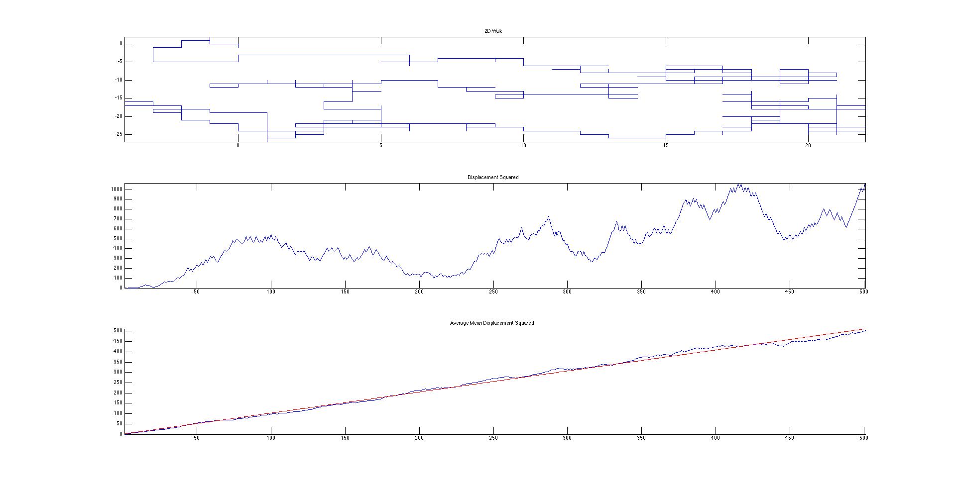
Figure 1. Drunken Motion in 2D. No variables.
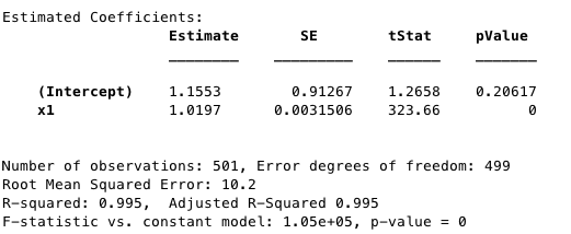
Figure 2. Statistics of Figure 1. Calculated with fitlm function of MATLAB.
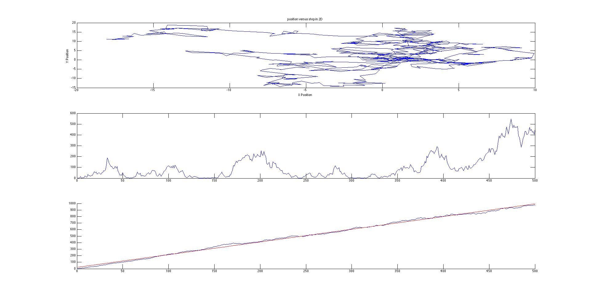
Figure 3. Brownian Motion in 2D
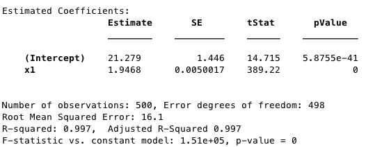
Figure 4. Statistics of Figure 3. Calculated with fitlm function of MATLAB.
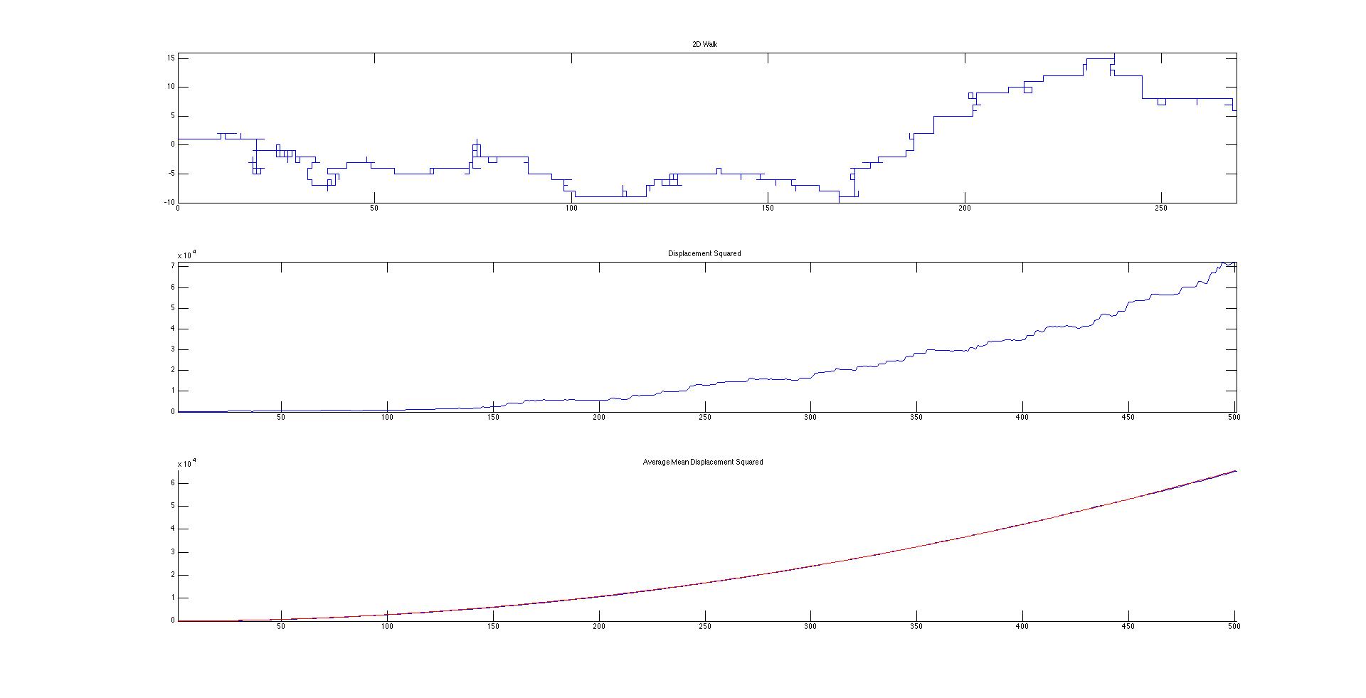
Figure 5. Drunken Walk with drift assigned with a 10% chance of taking 5 steps in +x or +y direction. fit=0.2550t^2+1.0161t+68.1101. R-squared=1.0000
Not only is drift visible on the motion map, the mean displacement squared is magnitudes larger between Figures 1 and 5. When drift was added, a second diffusion constant had to be added since the equation for mean displacement squared became parabolic. Since I am not comparing the mean squared displacements to a system with density (there is only one particle in my system), I can simplify the diffusion constants to be the slopes of their respective best fit lines. According to Figures 2,4, and 5, the diffusion constants are very precise and accurate (error is much less than 1% for linear diffusion), which indicate a statistically significant difference between the different walk methods.
The difference drift makes is considerable. This is important to keep in mind when considering chemical, biological, and physical systems. For example, a higher amount of drift, caused by a higher temperature or lower density on one side of a semi permeable membrane, alters solvent flux. Future directions for my experiment would be comparing the different sources of drift to each other. I would be very interested in modeling the real movement of solutes across a membrane under different gradients, such as temperature or solute density.
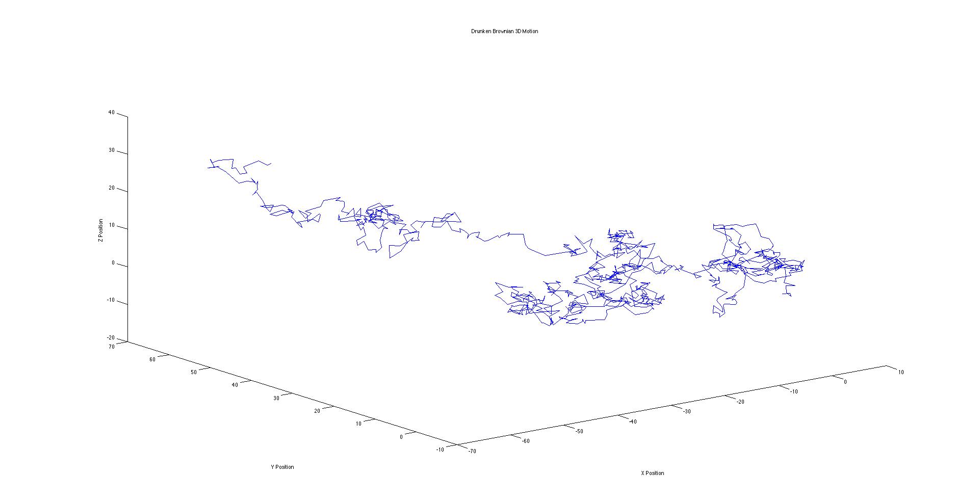
Figure 6. Brownian Motion in 3D. This isn’t all too significant to the rest of my project, but it is a visual representation of the path a liquid or gas molecule takes in a 3D homogenous box.
All 4 of my codes can be found here-https://docs.google.com/document/d/1nvyB5giUicIIiCJuKNKTwJagBlepP8J-IOQsMeMgB7Q/edit

Dillon,
It’s a bummer you didn’t get into the intricacies of the many variables that might arise in a drunken wander. It seems you might have benefitted from collecting more data outside of class! You built a really solid foundation of code to work on and introduced one variable, drift. The code you wrote has great potential to include these many variables you envisioned writing into the programs.
Your extension beyond the grid-like motion from your first random walk into Brownian motion was the most interesting part of this project. It was satisfying to witness the very clear change in the diffusion rates between the original random walk and Brownian motion. I would have liked to see some theory or equations behind Brownian motion if only to demonstrate some expected values/shapes of your diffusion rates when you changed walk methods. While your original goals were very different, I think this was the most interesting thing you demonstrated and I would have enjoyed more discussion. How does this extraordinarily simplified model of random particle motion compare to the actual behavior or diffusion rates? I am curious how and in what specific contexts, in your opinion, this sort of simple code could help us understand real phenomena.
To comment on your code, I was very impressed with how compact your Brownian motion routines were. Your use of “struct()” and the following code was a significant improvement in terms of how many lines of code it took to do the same thing with else-if statements (I realize this also has a lot to do with the nature of the type of motion you were modeling). Overall I was able to follow your code, but there could definitely have been a bit more commenting to explain your decisions/code. The final result is clearly different when you run each script, but when looking at them it is not immediately apparent they are much different. A header with a description of the code’s purpose and function would have been great, and I highly suggest it on future projects.
Fun project. Also the manner in which you had matlab spit out the final plots and subplots and data was very nicely organized.
Matteo
Drift is an interesting feature to incorporate in your model since it shows up in so many scenario’s. It would be nice to write out the meaning of your abbreviations like SE and TStats.