Introduction

Our initial plans for this project were to model and guitar string, piano string, and drum head in MatLab, then compare data calculated to a real scenario, using the physical instruments and recording the sounds they create.  We were able to complete the guitar and piano strings, but were not able to advance to the drum head due to time constraints.  However, we did get a lot of good data from our experiments with the guitar and piano strings.

Guitar String

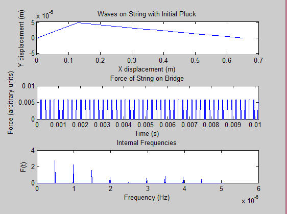
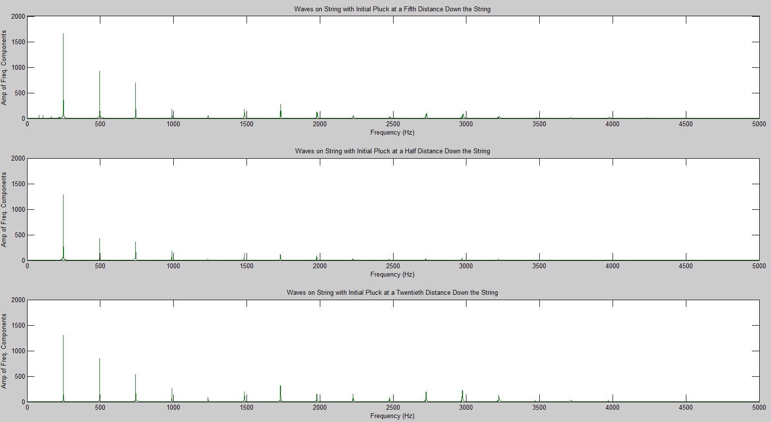
For this part of our project, we modeled a guitar’s B string in MatLab, and plucked the string at different points: once at the midpoint of the string, once 1/5 the string length from the bridge, and once 1/20 the string length from the bridge.  In the proceeding images, you can see the string oscillations, the force of the string on the guitar bridge with respect to time, and the Fourier Transform of these force graphs, which reveal the frequencies inside.

Modeled Guitar Data:

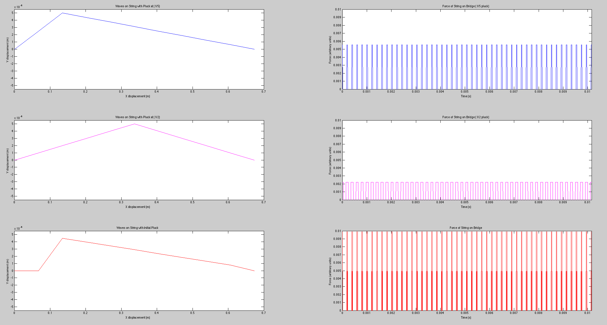
Frequencies of waveforms (Fourier Transform):

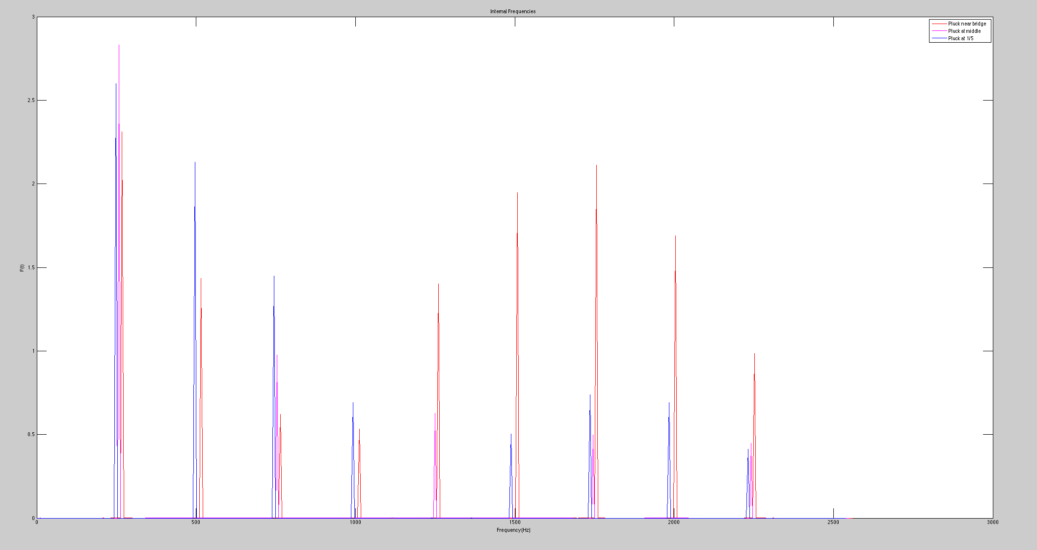
The force of the string on the bridge with respect to time is nearly identical to the sound wave that the string produces in the atmosphere, thus we were able to use that data to find the frequencies in our calculated string.  We also shifted the frequencies on the graph of the Fourier Transform for visual purposes (if not shifted, they would line up on top of each other and be difficult to distinguish).

Next, we recorded a guitar B string, identical to the one we modeled, and Fourier transformed those recordings to obtain the frequencies inside.

Frequencies of Physical Guitar String:

Here are the recorded guitar sound files.  Note as the pluck gets closer to the bridge, the tone of the guitar becomes harsher.  We will discuss this soon.

String Plucked at (1/2) distance:

String Plucked at (1/5) distance:

String plucked at (1/20) distance:

In our code for the modeled guitar string, the calculated waveform is played for the viewer, and as seen from the physical guitar, the tone of the sound gets harsher as the pluck gets closer to the bridge.  This harsher sound is the stronger presence of the overtones in the waveform as seen in our Fourier transforms.  As the pluck gets closer to the bridge, strength of the higher frequencies increases, which is why the sounds produced becomes much harsher.  This is what we expected and found with this part of the experiment.  Comparing our Fourier transform graphs, we see that the peaks at the higher frequencies increase with each pluck closer to the bridge.  We can also see that the closer the pluck is to the bridge, the lower the fundamental frequency becomes present in the produced sound.

However, there are some inconsistencies between the modeled and physical strings.  The modeled string did not contain and decaying properties, where the physical string did.  Also, the modeled string data was calculated using two dimensions when the physicals string would utilize all 3.   This important difference shows in the Fourier Transform of the modeled string.  When the modeled string is plucked at the halfway point, every other frequency (or peak) is eliminated from the Fourier transform; same as when plucked at 1/5, the fifth and tenth peak is eliminated.  In this modeled state, we are effectively killing these overtones by plucking where they would naturally occur on the string.  The decay properties of the physical string allow these “ghosted” frequencies to sound because the string can move freely rather than stay in a fixed 2-D dimension and fixed wave profile.  Another reason behind this, could be that the physical string is not of ideal form, meaning it is a series of coiled wires rather than a solid string.  This could have imperfections giving rise to these “ghosted” frequencies.

Another small discrepancy in our data is that the fundamental frequency of the physical string plucked at the halfway point is lower than when plucked at the other distances.  We don’t see this in our modeled system because the amplitude of the pluck was held constant for each pluck (giving us the results we expect).  On the physical string, the string is able to bend more at the middle than closer to the bridge.  Thus to get an equal volume pluck, we must do a harder pluck in the middle than closer to the bridge.  If we kept the amplitude of the plucks for the physical guitar the same, we would expected the power of the individual frequencies to closer match the modeled ones.

Piano String

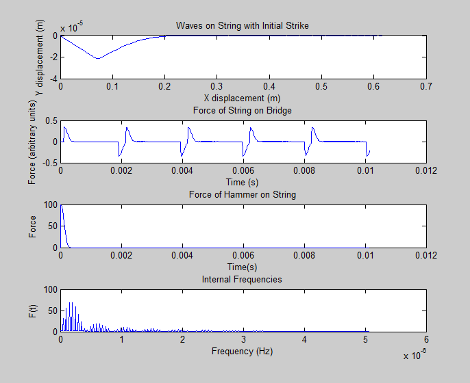
For this part of our project, we modeled a piano’s middle C string in MatLab, and struck the string with different forces: Once softly, and once more powerfully.  In the proceeding images, you can see the string oscillations, the force of the string on the piano bridge with respect to time, and the Fourier Transform of these force graphs, which reveal the frequencies inside, all for two different hit intensities.

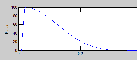
The model included a hammer with mass and an original velocity (which changes between the two trials) as well as a felt on the hammer which behaves as a spring. Here the compression of the felt is dependent on the position of the hammer and the string section where the hammer strikes, and which affects the positions of the freely moving hammer and string based on its compression. When the compression changes signs, we know that the hammer has left the string and we automatically give the string no outside force.

Modeled Piano Data and Frequencies

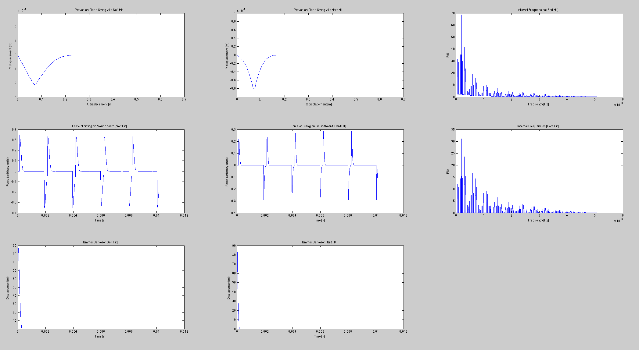
The force of the string on the bridge with respect to time is nearly identical to the sound wave that the string produces in the atmosphere, thus we were able to use that data to find the frequencies in our calculated string.

Next, we recorded a piano C string, identical to the one we modeled, and Fourier transformed those recordings to obtain the frequencies inside.

Frequencies of Real Piano String

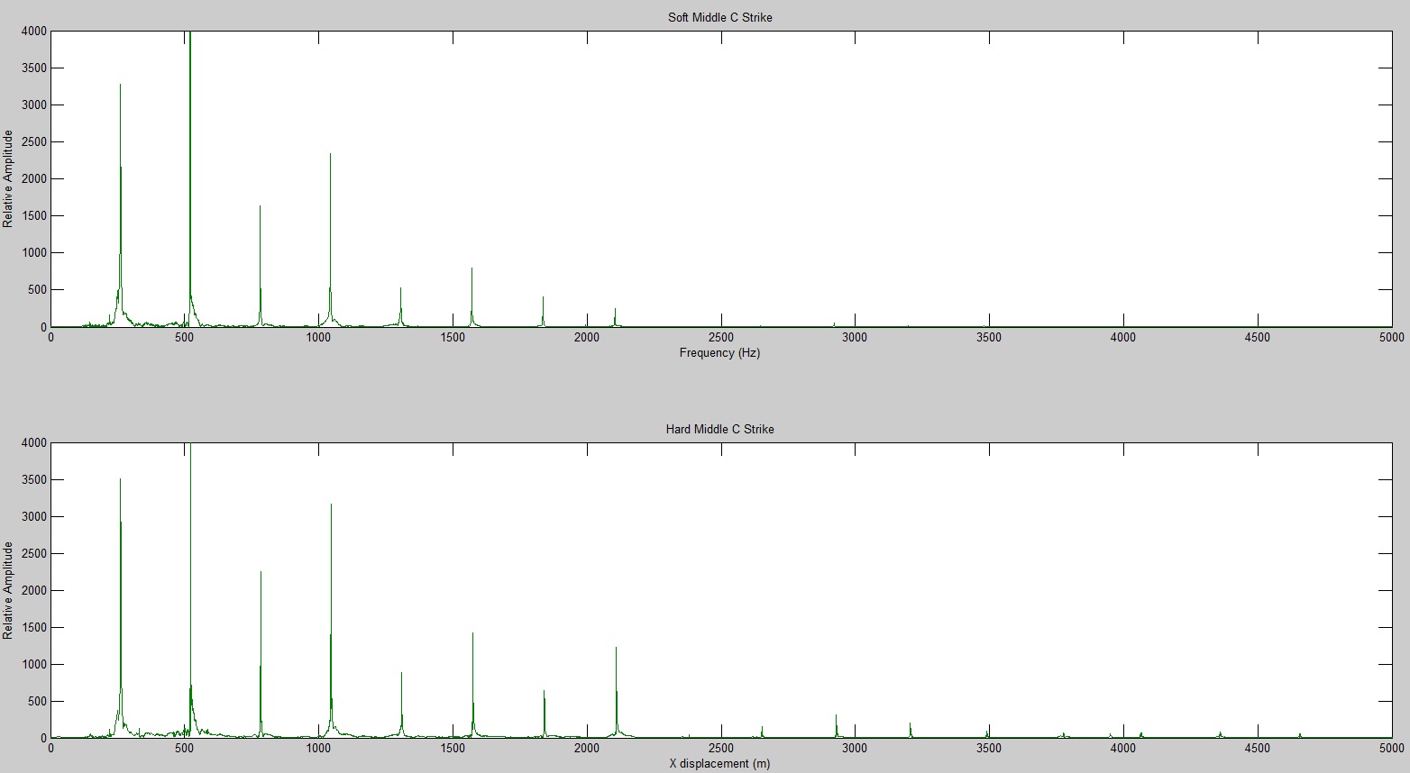
Here are the recorded piano sound files.  Note when the strike is harder, the tone of the guitar becomes harsher.  We will discuss this soon.

Hard String Hit:

Soft String Hit:

In our code for the modeled piano string, as the strike gets harder, strength of the higher frequencies increases, which is why the sounds produced becomes much harsher.  This is what we expected and found with our simulations.  A similar trend was also found in the Fourier transformed recorded sound files.

However, there are some inconsistencies between the modeled and physical strings. One such difference was the lower fundamental frequency than the second overtone in the recordings, as compared to our model. This could be due to the amplifying qualities of the piano box. The modeled string did not contain and decaying properties, where the physical string did.  Also, the modeled string data was calculated using two dimensions when the physicals string would utilize all 3.  The model we simulated made assumptions about the spring like qualities of the felt, the width of the hammer, as well as the strike intensity, which we couldn’t make equivalent to the recorded strikes. This created some strange differences, including a strangely sharp hammer hit (not as soft as one might expect from a spring, as well as differing from the textbook’s predicted hammer behavior). We brainstormed what may be it’s cause (the hammer velocity, the original felt thickness, the hammer’s strike position) but couldn’t find a solution.

Conclusion

In conclusion our results were what we expected with some degree of uncertainty. String plucks closer to the bridge and harder string strikes produce more overtone notes relative to the fundamental frequency. If we had more time/if this project were to continue further, we would explore the addition of a damping coefficient in our modeled experiments and compare with physical strings, investigating the discrepancies mentioned earlier.  We would also begin to explore the drum head dynamics, experimenting with two 3-D membranes, connected through a closed hoop, similar to the structure of an actual drum.

The following link is to a google drive containing all of our code and sound files.

https://drive.google.com/folderview?id=0ByhnW_B9B6q9flE5bWtTal9Yd19ZYzhrOGpUbjctMUhIM3FMRGxvMDVMZkF3NUJSbFJ1MEU&usp=sharing

Please note, if you are planning to run the code that involves the recordings of the instruments, YOU MUST CHANGE THE DIRECTORY IN WHICH THE CODE CALLS THE SOUND FILE.  Each space in the code is noted where this part should be edited.  This needs to be done as the naming of folders and drives varies from computer to computer.  Not only must the correct location of the file be used, but the sound files must be saved in the same location as the MatLab code or it will not run.  Also the correct sound file must be called in each spot, or the sampling will be off/ the code will not run properly.

The piano string is a much more difficult scenario to model than the plucked guitar string.  The guitar string is a pluck, which can be easily modeled with an initial string position.  The piano string has a felt covered hammer that strikes the string, then a standing wave will form.  Seen in the data below, we were able to construct an initial hammer strike on the string, and analyze how it moved throughout:

Our force on the bridge diagram yielded a decent fourier transform but we came across one problem, our hammer string was not executed properly.  In the class text, the force of the hammer on the string, with the spring force behavior from the felt, should yield a soft hit that should appear as a parabolic force vs. time diagram.  Our data shows that it increases linearly and then proceeds to decrease at an acceptable rate. This is something that we must look further into.

Hammer Force seen in class textbook: (Computational Physics, Giordano, p.366)

(image to be added)

Hammer Force we calculated:

This needs to be re-evaluated in order to compare when testing and recording with a physical string.

Link to code: https://docs.google.com/document/d/1tNIwInru6_DcevXB49tW-0ULWkmS8BH2hKv6Tyn9kY4/edit?usp=sharing

Here is the code for our modeled guitar string and the resulting force on the bridge.  This force oscillates with time, similar to the frequency of the sound waves that the instrument produces.  We were able to find the base and overtone frequencies using the fast fourier transform function in MatLab, however our scaling is off for graphing purposes.  However, we know our data is correct because we plucked the string at a distance (B=1/5) of the total length of the string which resulted in our fourier transform missing a 5th peak.  For future testing, we hope to record a physical string with similar variables to the one in our code, import the sound file to MatLab, analyze the frequencies, and compare it to the results of the modeled string.

——————————————————————————————————————————————

Link to code:

https://docs.google.com/document/d/1vNhrcuUVjmwfNM8raGKmyKAl0Z19bFR8c7rikb9tI1w/edit?usp=sharing

close all
clear all
%%%GUITAR STRING%%%

%% Initialize Variables
L=.65; %Length of string (m)
T=149; %Tension of string (N)
c=320; %Velocity of wave (m/s)
dx=.065; %Distance step
dt=0.00001015625; %time step (s)
r=1; %constant in oscillation calculation equation
Amp=.000005; %Amplitude of pluck (m)
Lpluck=.13; %Length of pluck spot (m)
B=Lpluck/L; %pluck position on string (m)
M=[0]; %Array for y vaules
runtime=1000;

%% Builds initial pluck array
for i=dx:dx:Lpluck
y=i*Amp/Lpluck;
M=[M,y];
end

for i=(Lpluck+dx):dx:L
y=(i-L)*(-Amp/(L-Lpluck));
M=[M,y];
end

%% Build X-aixs
x_axis=[];

for i=0:dx:L
x_axis=[x_axis,i];
end

%% Initialize Loop variables

ynew=zeros(1,length(M));
ycurrent=zeros(1,length(M));
yold=zeros(1,length(M));
ycurrent=M;
yold=M;

F=[];
N=[];

%% Animation Loop (String Oscillations)

for n=1:runtime

for i=2:length(M)-1
ynew(i)=2*(1-r^2)*ycurrent(i)-yold(i)+(r^2)*(ycurrent(i+1)+ycurrent(i-1));
end

f=T*(ynew(2)-ynew(1))/dx;
F=[F,f];

N=[N,(n*dt)];

yold=ycurrent;
ycurrent=ynew;

subplot(3,1,1)
plot(x_axis,ynew)
axis([0,0.7,-Amp*1.1,Amp*1.1])
title(‘Waves on String with Initial Pluck’);
xlabel(‘X displacement (m)’);
ylabel(‘Y displacement (m)’);

subplot(3,1,2)
plot(N,F)
axis([0,runtime*dt,0,0.01])
title(‘Force of String on Bridge’)
xlabel(‘Time (s)’)
ylabel(‘Force (arbitrary units)’)

pause(0.000001)
end

%% Tension/Frequency

FFT=fft(F);

FTscale=2^nextpow2(runtime);
f=dt/2*linspace(0,1,FTscale/2+1);

subplot(3,1,3)
plot(f,(2*abs(FFT(1:FTscale/2+1))))
title(‘Internal Frequencies’)
xlabel(‘Frequency (Hz)’)
ylabel(‘F(t)’)

%need to fix scale on FT

Physics of Musical Instruments Project Plan

Greg Cristina, Teddy Stanescu

Objective:  Explore the physics behind the sound of different musical instruments; vibrations through different mediums and the frequencies they create. We will be looking to experiment with these three musical instruments:

1. Guitar (a plucked string)
2. Piano (a hammered string)
3. Drum (a hammered membrane)

Chapter/Section(s) of Focus: We will focus on theory and use equations from Chapter 11 in the class text (Giordano), specifically sections 11.1, 11.2, and 11.4.

Overview: We want to model each of these 3 instruments in Matlab, using the computational methods and equations provided in the text.  These models will consist of the physical behavior of the instruments, such as (x,y,z) displacement of a string/membrane at a given time t and the frequencies/harmonics (overtones) they produce given specified initial conditions.  From here, we will take advantage of Matlab’s ability to read and extrapolate data from audio files by mimicking our theoretical scenarios modeled in Matlab as a physical test, using the actual instruments, keeping as many initial parameters as possible constant.  We will record the sound produced by the instruments using a microphone and recording software (audacity/reaper), import to Matlab, and compare the recorded data to the data calculated through the computational methods.

Experimentation:  For the guitar string, we will pluck the string at different distances from the bridge.  For the piano string, we will strike the string with different strength forces from the hammer.  These changes in how the instrument is played are shown in the text to yield different frequencies and harmonics, and we will further investigate this phenomenon.  The drum will be the biggest challenge to experiment with because there is no direct example in the text.  However, it covers many methods that we will modify and test such as relating the force of a guitar or piano string on the soundboard to the frequency it produces.  Also, the text has a banjo example of how a wave on a string affects a membrane and the frequencies they produce, which is similar to the two heads of a drum interacting with each other to produce a sound.  Using knowledge gained from experimenting with the guitar and piano strings, we will investigate drum membrane physics and attempt to model in Matlab, if model is successful, a recording with be made and compared.

Sources used (as of now):

–Computational Physics, Nicholas Giordano

-more to come if necessary

Timeline:

Week 1 – Model guitar string in Matlab, and test at different distances from bridge.

Week 2 – Model piano string in Matlab, and test different hammer forces

Week 3 – Record guitar and piano string, analyze and compare with Matlab calculated data

Week 4 – Drum experimentation

Week 5 – Organize data in a presentable manner, fix any errors in data analysis