Precession of Mercurian Planets: Data and Results

Over the past week I have developed my code to achieve a fairly accurate approximation of Mercury’s precession due to the general relativistic effects of the sun. This was achieved by plotting the orbital motion of Mercury over 7 orbital periods, then saving the locations of the perihelions from each of the orbits. From these perihelions, I was able to graph the precession rate, $\frac{\delta(\theta)}{\delta(t)}$ . For an alpha of 0.0015:

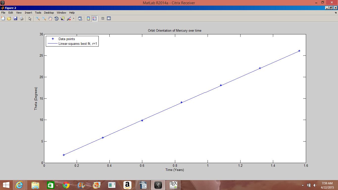
The slope of the linear-squares best fit gives the rate of precession experienced by Mercury at this value of alpha. In order to extrapolate the true precession rate of Mercury (which is very small and would be difficult to calculate using the above method) by graphing the precession rate as would be experienced by Mercury at different values of alpha. (As seen previously, precession rate is given by C*alpha; the relationship between precession rate and alpha should be linear. For Mercury this resulted in the graph:

The slope of this graph (C) was calculated to be $1.1997*10^{4} \frac{degrees}{year*unit alpha}$ ; which is close to the true value, $1.11*10^{4} \frac{degrees}{year*unit alpha}$ . This yielded a precession rate of $47.4685 \frac{arcseconds}{century}$ , as compared to Mercury’s true value, $43 \frac{arcseconds}{century}$ . This corresponds to a percent error deviation of about 10.39.

After completing this extrapolation, I began an investigation into the effect of eccentricity on the precession of the perihelion of a planet’s orbit. I left the both the mass and perihelion values for my test planet to be the same values as for Mercury, however I allowed the semi-major axis length and eccentricity values to vary. Holding the perihelion constant at the value of Mercury’s perihelion results in the expression $e=1-0.31 \frac{AU}{a}$ , where e is the eccentricity and a is the semi-major axis length in astronomical units. Using the same method as given above, I was able to calculate the precession constants C for 7 different Mercurian systems, each with a different value of eccentricity. The results are shown below:

As can be seen by the graph, the best fit for this set of data is a multiple-linear regression fit, of degree 2. Checking this result with Einstein’s expression for the precession rate:

$\epsilon=24*\frac{(\pi^{3})*(a^{2})}{(T^{2})(c^{2})(1-e^{2})}$

We see that the precession rate is indeed inversely proportional to $e^{2}$ .

Here is a link to my updated Mercury Precession code:
https://docs.google.com/a/vassar.edu/document/d/1fw8L5ZvhqMMVMYltkJH6Ac425KrmnbbDUJs_6GV7aPI/edit?usp=sharing

And a link to my Mercurian Eccentricity code:
https://docs.google.com/a/vassar.edu/document/d/1eqEBSExnBQZRgFUq9GYQDdjTqC9EODRIR0llXQv7sMw/edit?usp=sharing

References:

Computational Physics by Nicholas J. Giordano and Hisao Nakanishi

Vankov, A.A. “Einstein’s Paper: Explanation of the Perihelion Motion of Mercury from General Relativity Theory”.

Modeling and Experimental Tools with Prof. Magnes

Ideal for getting ideas and feedback on upper level physics tools.

1 thought on “Precession of Mercurian Planets: Data and Results”