Sushant Mahat

Mohammed Abdelaziz

Since last week, we have managed to greatly fine tune our program, and get more data.

We are using the same basic functions we created last week: TheInitiator and TheUpdater. However, as mentioned in the earlier post, our TheUpdater function was not functioning ideally. The profile of the Lennard-Jones potential is such that when two particles get close together (less than ~1.1 reduced unit in length), they exert a large repulsive force on each other and send each other moving away at large velocities. If you look at the Lennard-Jones potential in Figure 1 below, you can see that the force changes from attractive to slightly repulsive to extremely repulsive very fast (force changes by ~100 reduced units of force over ~0.3 reduced units in length). In real life, two particles repel each other before they get this close, so the force should never become very large. However, our function discretizes time, so there is a small chance that particles get very close to each other before they feel the repulsive force. This creates a repulsive force that catapults one of the particles, which breaks the law of energy conservation. The catapulting effect decreased when we decreased the time step dt (our discretization in time), but it did not go away completely.

To solve this problem, we divided TheUpdater into two parts: TheUpdater and TheEnforcer. TheEnforcer function calculates the force between each pair of particles and the total force on each particle. However, this function is designed such that if two particles accidentally get close to each other during dt, the force they exert on each other will be limited to a certain value (i.e. we cap the max force). We think this change is valid as two particles, with the velocities we use, would never get so close that they would exert more than our max force on each other. Apart from that, we have also made changes to the net force direction. In our last program, we were able to determine repulsive or attractive forces but it turns out we made an error in translating this information to force in the x direction and the y direction. This is especially hard as we have periodic boundary conditions, so it is not always clear whether a particle is “to the left” or “to the right” of another particle, for instance. However, we are confident that we have managed to get the force direction correct this time. We tested it by running a program with just 5 particles in a small box (size of 10* 10), so that it would be easier to monitor their interactions. During our several runs, we saw several different interactions where our particles curve around each other and attract at certain distances and then repel, as expected, which is a significant improvement to our last program. Video 1 showcases this test.

TheUpdater function now calculates positions and updates the velocity of our particle using the output from TheEnforcer. These data are fed into the main body script which calls upon another function: SpeedDist. SpeedDist finds the speed distribution of our particles. Figure 2 below shows that the average speed remains very close to 1 reduced speed unit, which was our initial average speed. In the coming weeks, we will also include another plot that shows the kinetic energy of all particles with respect to time, and the cumulative Kinetic energy of all particles. This information will be interesting because it can directly be used to calculate the temperature of the system, potentially allowing us to test the effects on the system when we manipulate the temperature.

Figure 1. This figure shows the Lennard-Jones potential. The x axis is length in reduced units. The reduced unit of length is based on the size of an argon molecule. The steep increase in potential below a distance of 1 suggests a rapid increase in repulsive force as two particles come close to each other. This essentially creates a “hard sphere” around each particle.

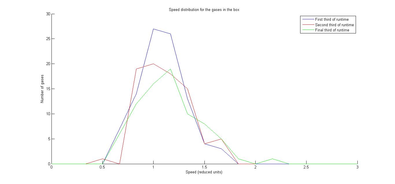
Figure 2. Speed distribution of 100 particles in a 25*25 box. The average speed remains roughly constant over the time interval and closely resembles Maxwell distribution. The total time for the simulation was 10 reduced time units where 1 reduced time units is approximately 2 picoseconds.

Video 1. This is a video of 5 particles in a  10*10 box. You can see the particles interacting in several ways.

Video 2. This is a video of 25 particles in a 10*10 box. It demonstrates that the interactions still work for greater numbers of particles (we have found that even simulations of 200 particles can be calculated in under a minute).

A note on reduced units:

Reduced units are used for convenience and simplicity in the equations used for the simulations because they avoid the need of having to put constants in every calculation. We have been somewhat vague about what each reduced unit represents in terms of common units, but will explicitly define these in a future post.

Edit (4/27/15):

We forgot to upload our most recent working script and functions; they can be found here.