Author Archives: tekpulun

Conclusion-Brian and Tewa

Outline:

1. Questions from Comments

2. Analysis of our Neural Network

3. Concluding Remarks

4. Future Plans

1. Questions from Comments:

In this section, we will be answering the questions we received from our last post.

  1. It seems that not every neuron is connected to EVERY other neuron since there are different connection pattern.
  2. When you say an energy of “-5000″ what are your units/reference point?  I am still wondering how and why the Monte Carlo Method works and how the energy state is so low for ordered systems.  This may be unrelated and somewhat random, however, why is it that entropy (disorder) in chemistry always increases and is actually considered a lower state of energy?

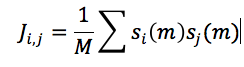
Every neuron in our neural network is connected to one another. The results of their connection can be found within the j-matrix; each pattern has it’s own j-matrix.  When we store multiple patterns in one system, separate J matrices are created for each pattern, but the J matrix that is used (J_total) is the element-wise average of the separate J matrices.  So, for each neural network there is only one J matrix, which describes the connections between each neuron and every other neuron.

When a pattern is greatly distorted it takes more energy to return it back to the desired pattern. However, entropy states that the greater the disorder the lower the state of energy. Our neural network is an artificial system that has no relations to entropy. Our energy state for ordered patterns is less than that of disordered patterns because that is the way our code is designed. Furthermore, our j-matrix is designed so that when we calculate the energy of stored patterns it gives us a large negative value for energy. However, when we calculate the energy of disordered patterns it gives us energies close to zero.  The energy calculated in our neural network does not have units; it’s similar to intensity where we are just concerned with the relative energy between the neurons. The Monte Carlo method simply goes through a distorted pattern and determines whether or not a neuron needs to be flipped. This decision is based on the input of one neuron from the summation of the inputs of  the other neurons within the neural network.

2. Analysis of our Neural Network:

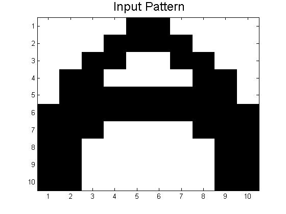
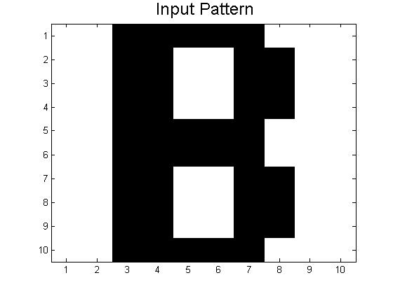
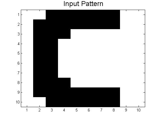
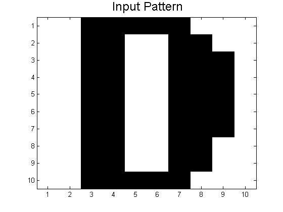
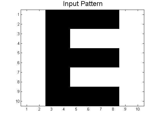
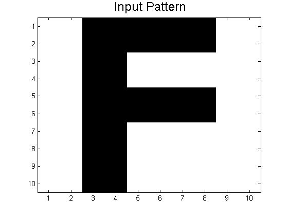
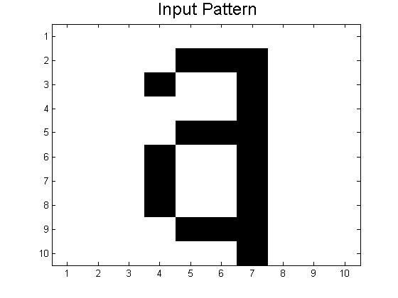
Since our last post we have created neural networks with a larger number of patterns stored, in an attempt to study the system as it begins to fail correct memory recall.  The way we accomplished this was by building systems with more letters as stored patterns.  We had a system which stored A-C, one which stored A-D, and one that had A-F and also a lowercase letter a.  Pictures of all of the letters we used as stored patterns are shown below.

Below are the 7 stored patterns within our neural network.

input_A  input_B  input_normal_C  input_D  input_E  input_F  input_little_a

These systems (and links to their codes) are discussed below, but first a little background on the storage of many patterns in neural networks.

As explained in our previous posts, storing more patterns in a neural network causes these patterns to become more unstable: if you think of the energy energy landscape picture from our last post, the minima associated with each pattern become shallower the more patterns that are stored.  This occurs because of the averaging of all the J matrices that correspond to the individual patterns that we want to store: each new pattern distorts parts of the other patterns.  This can be seen visually in the pictures of the J matrices in our last post; the combination of A and B is much more complicated than A and B on their own.

Our textbook (Giordano and Nakanishi) talks about the limitations of how many patterns can be stored in a neural network.  The main obstacles are that 1. any patterns that are too close to each other will likely interfere, and 2. there is a theoretical limit at which the system changes and all patterns become unstable.

For 1., think of the energy landscape again, as well as the letters we use.  The minima for the letters B and D will be relatively close together on the energy landscape because they are relatively similar patterns, and thus their troughs will likely merge a bit and may produce patterns somewhere between the two.  We run into exactly this problem with our A-D code, which often works for A and C (as long as they are not too distorted, usually less than 0.3 or so), but which usually returns a pattern somewhere between B and D when given distorted inputs of B or D.


input_distorted_D_0.05  output_distorted_D_0.05

If you want to try this out for yourself, use the code below.

Link to Code: Stored Patterns A-D

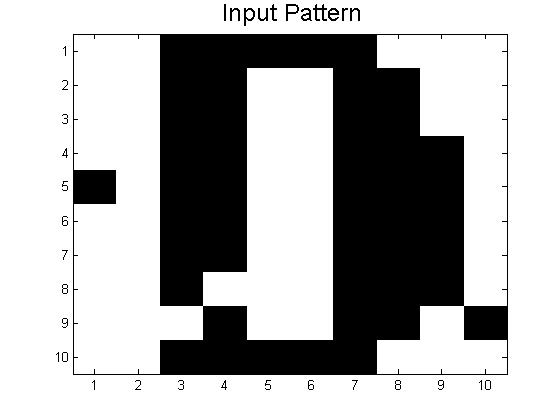
The theoretical limit of the number of patterns that can be stored is given in the text as ~0.13N (in our case, 13 patterns).  Our neural networks begin to function very poorly once we store 7 patterns (A, B, C, D, E, F, a); beyond simply confusing the letters that are similar, nearly all inputs lead to the same answer, a strange hybrid of letters (mainly F and B it seems), shown below.

input_normal_C  output_weird_F_B_hybrid

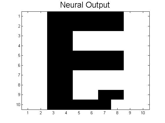
This code actually does work for some inputs (if given an A distorted by 0.1 or less, successful recall of the letter A is usually achieved).  However, nearly all inputs, even those unlike any other pattern (such as the lowercase a) give the same jumbled result seen above.  This is likely a combination of the two effects mentioned above: many patterns here are similar to each other, and the number of patterns has significantly lessened the deepness of the minima associated with each pattern, leading to more instability across all of the stored patterns.  Ideas for how to get real systems closer to this theoretical limit of 0.13N are discussed in Future Plans.

Try this out for yourself with code below.

Link to Code: Stored Patterns A-F + a

We were able to create a very functional neural network that stored three patterns, A-C, which avoided almost all of the problems of having patterns too similar to one another and having so many patterns that the energy landscape minima become too shallow.  The link to this code is below.

Link to Code: Stored Patterns A-C

3. Concluding Remarks:

We started this project in wanting to answer these questions:

    1. How far away initial inputs can be from stored patterns while maintaining successful recall.
    2. How many patterns can be stored in the neural network.  The book discusses the maximums associated with this type of neural network, but we will investigate why this limit exists, as well as what kinds of behaviors change around this limit.
    3. How long (how many Monte Carlo iterations) recall of stored patterns takes.

During the time spent on this project we were able to answer the above questions. However, we also ran into several unexpected problems and results. We found that the most we could distort a pattern is by roughly flipping 45% of the pattern, in order for our code to still work. Patterns that were distorted by 50% no longer worked and the image output was not recognizable. These numbers are based on a neural network with just three patterns: A, B, and C.

Several patterns can be stored in the neural network, however in order to have a neural network that works, we could only store 3 of our 7 patterns. This is so because after C, the letters become very similar to one another; for instance B and D or E and F. With these similarities the neural network produces output patterns that are half way between the similar letters, instead of one letter.  If we had 7 patterns that were all drastically different from one another, we believe that our neural network would work.

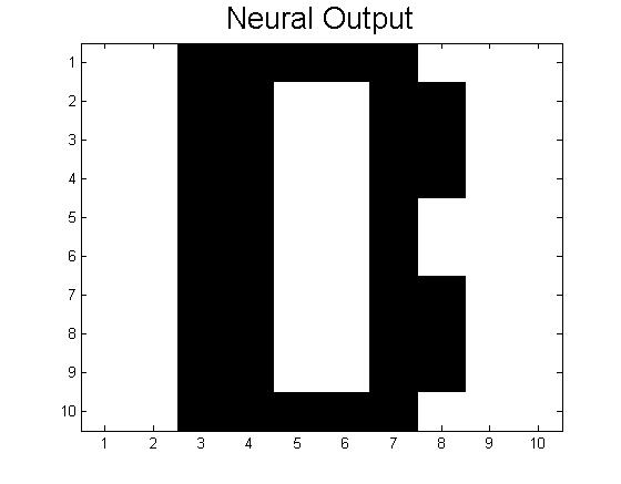
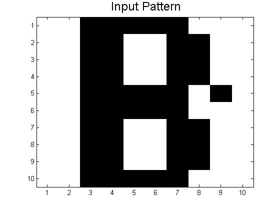
The amount of Monte Carlo iterations is highly dependent on the amount of patterns stored in our neural network and by how distorted a pattern is. In our code we set a limit of 1000 iterations where the program stops if it is taking 1000 Monte Carlo sweeps to achieve the desired pattern. If a program takes 1000 iterations it means that the desired pattern we want is not going to be produced. This is where you get patterns that are incomplete or half way between two letters. When our neural network was successful it only took 1 Monte Carlo iteration to give us the desired pattern. Below is a picture of a distorted B and the output result after 1000 iterations, which is a pattern between B and D. As you can see the distorted B is very close to  the letter B, however because this neural network has D stored as a pattern, it can not make up it’s mind as to which letter to display.

input_distorted_B_0.05   output_distorted_D_0.05


4. Future Plans:

One of the main things we would want to do next is to create a neural network with more patterns, approaching that theoretical limit of 0.13N.  The best way to do this is likely with patterns that are more orthogonal than the letter patterns we used in this project.  This would be easiest to accomplish with very simple but drastically different patterns, such as vertical lines or circles in different positions.  With these new patterns, we would be able to uncover much more about our neural network than we can now with storing letter patterns that are very similar to one another.

Another objective we would want to tackle is how the size of the neural network affects its function.  Specifically, I wonder if we used the same 7 patterns (letters A-F and lowercase a) but in a neural network that was 15×15 neurons (or even bigger), would we be able to get successful recall of the lowercase a, as we were unable to with our current 10×10 size network?  More neurons (more importantly, a bigger J matrix) should be able to handle more patterns before the energy landscape minima become too shallow, so this should work, in theory.  Testing this would provide us more insight into the limitations on the number of patterns that can be stored in a neural network.
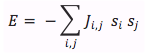
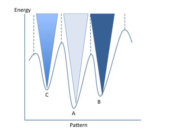
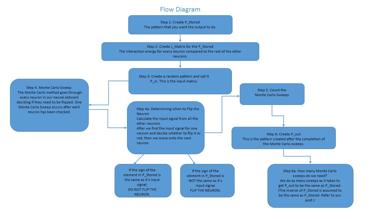
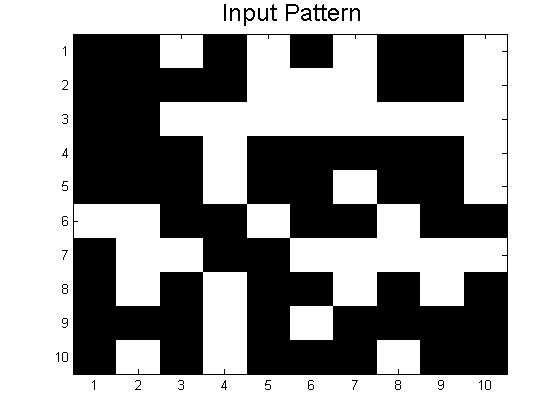
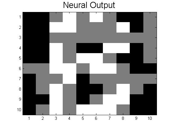
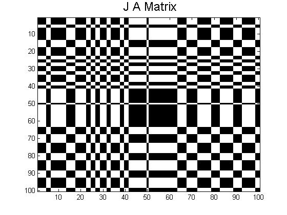
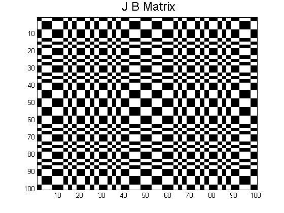
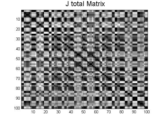
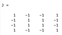
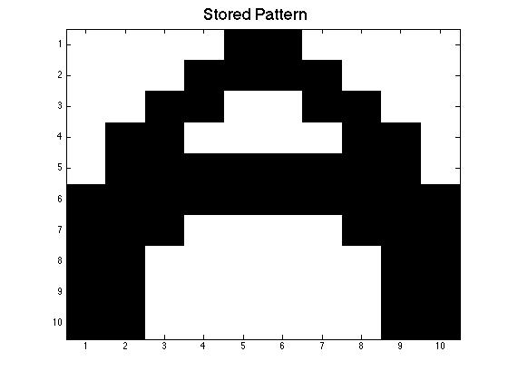
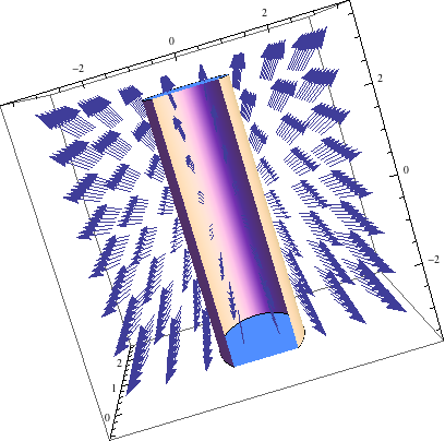
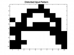
Share

Brian and Tewa – More Data and Analysis of Neural Networks

After some more investigation of our Neural Network model, we have refined our Monte Carlo flipping rules, have stored more than one pattern in our neural network, and have determined that, effectively, the inverse of a certain pattern is equivalent to the initial pattern (they both are energy minima).  Before we delve into these results, we will clear up some questions about our original data post.

Outline:

1. Physics from Statistical Mechanics?

2. A Neural Network

3. Monte Carlo Method

4. Project Goals

5. Constant Energy?

6. Flow Diagram

7. Energy Values

8. Flipping Conditions

9. User Friendly Code

10. Unique Random Pattern

11. J-matrices for A, B,  and their average


  1. Physics from Statistical Mechanics?

The model that we are using, the grid of neurons that are either in position +1 or -1, is very similar to the Ising Model (introduced in Chapter 8 of our text), but with some modifications that make it appropriate for modeling brains.  The Ising Model was originally created for studying the magnetic spins of solids and how they interact at different temperatures to explain ferromagnetism vs. paramagnetism, and how those change with phase transitions.  In this model, physics from statistical mechanics is used to see how the magnetic spins interact with a heat bath (temperature is non zero), as well as how they interact with each other: sometimes the spins will flip randomly because of heat bath interactions.  Our neural network model is essentially the Ising model with temperature equal to zero: our neurons never flip randomly on their own, but only in response to their connections with other neurons.  So our model does not use any physics from statistical mechanics, but uses a technique (the Monte Carlo method, which decides whether or not neurons (spins) should be flipped) that is used for many other applications as well.

  1.  A Neural Network 

A neural network, in our model, is a grid of neurons (which can have value +1 or -1 only, on or off, firing or not firing), which are completely interconnected (each neuron is connected to every other neuron).  The J matrix is where the connections between neurons are stored, and so the “memory” of the system is contained in the J matrix.  Patterns can be stored in these neural networks, and, if done correctly, stored patterns can be recalled from distorted versions of them.  The way that the neural network travels from the input pattern to the output pattern is via the Monte Carlo method.

  1. Monte Carlo Method

The Monte Carlo method is essentially just a way of deciding which neurons to flip, the goal, in this case, being to change the input pattern into one of the patterns that have been stored in the neural network.  The Monte Carlo method checks every neuron, decides if it should be flipped based on certain flipping rules, flips if necessary, and then goes onto the next neuron.  Once every neuron has been given the chance to flip, one Monte Carlo sweep has been done.  The details of the flipping rules depend on the model.  The flow diagram of our general code (in post below) explains our specific Monte Carlo flipping rules in greater detail.

For our neural network, we want to keep doing Monte Carlo sweeps until the output is equal to one of the stored patterns, which is when we say that the pattern has been recalled.  We also want to keep track of how many sweeps it takes to get there, because this is some measure of the speed of the system.  The flow diagram again goes into greater specific detail.

  1. Project Goals

Our goal in this project is to investigate the neural network model presented in the text.  First we had to get it working in the first place (meaning we had to be able to store and successfully recall patterns in a neural network), and then we planned on investigating the properties of this model, such as how long memory recall takes for different patterns and different systems, how many patterns could be stored in a single neural network at the same time, how performance of the network changes as more patterns are stored, etc.  How many of these questions we will get to by the end of this project is another story, but we will do our best.


  1.  Constant Energy?

The energy of the system, calculated with Equation 12.14 in the text

Screen Shot 2015-04-13 at 1.09.35 AM

is different for each different state that the system is currently in.  The way that the whole neural network stores patterns is the way that the J matrix is created.  It is created in such a way that the desired stored pattern(s) are energy minima of the system.  Because our Monte Carlo method flips neurons in a way that lowers the total energy of the system, our process should drive P_in towards one of the stored patterns, and stop once it reaches a minimum.  Figure 1 (inspired from figure 12.30 in the text) is helpful for visualization of this energy minima concept, and how stored patterns “trap” the Monte Carlo method and prevent the pattern from changing with further sweeps.  When the Monte Carlo method reaches one of the minima and finds a stable pattern (which is almost always one of the stored patterns, or its inverse (discussed below)), it cannot escape from this energy minima.  If this minima is equal to one of the stored patterns (or its inverse, discussed below), then our code stops and displays the output.  When this happens, we say that our system “recalled” the output pattern.  We also have a condition that stops our code after a large number of Monte Carlo sweeps (1000) and displays the output, regardless of whether or not recall was successful.  This is needed because sometimes the code gets stuck in a shallow energy minimum that is not equal to one of the stored patterns or one of its inverses.  In this case. we want to still display our results and see what went wrong (what pattern our neural network got stuck on).

Slide1

Figure 1: Schematic energy landscape. Each energy minima represents one of the stored patterns. When we give our neural network a specific pattern it produces a pattern with the same or lower energy than the initial pattern.


6.   Flow Diagram

The attached flow diagram provides a step by step guide for our code. This diagram also explains how our neural network functions when performing pattern recognition.Slide1

  1. Energy Values

We created a code that calculates the energy value for our stored patterns, their inverse, and a randomly generated pattern. Within this code (Energy Calculating Code) you can determine the minimum energy required to flip the neurons from active to inactive or vice versa within our neural network. We want the minimum energy value because this means that our neural network doesn’t need to exert a lot of energy in order to perform pattern recognition.

The energy minima for the stored pattern is much more smaller than that for the randomly generated pattern. This is so because our stored patterns have an order about them that the random pattern lacks. The energy values for the stored patterns and their inverse is -5000.The energy values for the random pattern is always greater than -5000 and close to but never greater than zero.

Furthermore, because the energy minimums are the same for both the stored patterns and their inverses we can assume that the stored pattern and its inverse are the same. In other words, our code starts of with black-blocked letters and the inverse is white-blocked letters. Although, white and black are two different colors, they represent the same letter, due to both of them having identical energies. This phenomenon occurs because if we distort the stored pattern by 80-90% it takes less energy to get to the inverse image than to the proper image, thus the inverse image is displayed as our P_out. In order to avoid this confusion, we set a condition that changes the inverse image back to the proper image.

Link to code: Energy Calculating Code

  1. Flipping Conditions

As illustrated in our flow diagram, the flipping conditions determine whether or not the neuron is flipped from inactive to active and vice versa. An input signal is calculated for each neuron and the sign of that input signal is compared to the sign of the neuron. If the signs for both are the same then that neuron is not flipped and remains in it’s current state. However, if the signs are not the same then the neuron is flipped to the state that corresponds with the sign of the input signal.

The input signal is telling the neuron which state to be in. For instance, if the input signal is greater than zero, it is telling the neuron to be in the positive 1 state or if the input signal is less than zero, it is telling the neuron to be in the negative 1 state.

9.User Friendly Code

This code allows for user input to determine which of a variety of input patterns P_in to investigate.  The choices for possible input patterns are listed below (and in comments in the code, if the user forgets):

  • P_A and P_B are simply equal to the stored patterns
  • negP_A and negP_B are the inverses of the stored patterns
  • distP_A and dist P_B are distorted versions of P_A and P_B, distorted by an amount input by the user
  • Rand is a random pattern of roughly equal amounts of +1 and -1’s
  • Rand_weird (half-way pattern) is a specific randomly created matrix that gets our code stuck, and we don’t know why…

Rand_weird is a specific instance of an input pattern where weird things happened, discussed more in the next section.

Link to Code: User Friendly Code

10.  Unique Random Pattern

While we were checking our randomly generated code, we ran into one unique pattern; let’s call it the half-way pattern. The half-way pattern can be assumed to be torn between becoming an A or a B. Because of this, no matter how many Monte Carlo sweeps the half-way pattern goes through, it will forever be torn between the two set patterns. The half-way pattern is the only randomly generated pattern, so far, that has an output where the half-way pattern displayed gray blocks; where the gray blocks represent the number 0. Remember the only two states we have for are neurons are positive and negative one. This gray output has an energy minima of -1745.

input_rand_weird      output_rand_weird


11. J-matrices for A, B,  and their average

Here are the J-matrices created by the pattern A, pattern B and then an average of the two. As you can see there are some patterns within each J-matrix, however it is not a reoccurring pattern. This means that there are certain patterns within each section of each J-matrix. J A Matrix      J B Matrix


J total Matrix


Share

Neural Networks: Preliminary Data – Brian Deer and Tewa Kpulun

As we began our project, we realized that the Ising model presented in Chapter 8 of Giordano and Nakanishi quickly introduces many aspects that are not relevant to our neural network model, namely the idea of a heat bath at temperature T.  Our neural network is essentially an Ising model assumed to have a temperature of 0, so much of Chapter 8 is unnecessary for our model.  So we skipped ahead and went straight to simple neural networks, as described in Section 12.3 of the text.

The essential elements of our model are an NxN stored pattern, an interaction matrix Ji,j of size N2x N2, and an input pattern of size NxN.  After a pattern is stored (by creating the network’s interaction matrix), an input pattern (usually one similar, but not identical, to the stored pattern) is presented.  This pattern is then changed according to the Monte Carlo method, and, if things worked correctly, the output is the same as the stored pattern.


Stored Pattern:

We created a stored pattern on MATLAB by creating a matrix +1’s and -1’s.  Our first pattern is the letter ‘A’, following the examples in Section 12.3 of Giordano and Nakanishi, on a 10×10 matrix.  As mentioned in our earlier posts, each element in the matrix represents a neuron and if the neuron is active it has a value of 1 and if it is inactive, its value is -1. Our ‘A’ pattern is made up of +/-1s where the +1’s represent the pattern and the -1’s represent the background. When these numbers are displayed in the command window, the A pattern is not easy to see, so we use the imagesc command (along with an inverted gray colormap) to better visualize our patterns.

Element Indexing

MATLAB indexes the elements in a matrix with two numbers: the first index refers to the row of the matrix, and the second index refers to the column.  For our neural networks, we want to be able to access every element in the array (twice, separately) in order to have every neuron interact with every other neuron.  The easiest way to do this is by using a single number index, i, which runs from 1 to  N2.  In our code, we use i and j.  To actually access the elements in our matrices, we have to use the normal double MATLAB indices, which we call call y and x.  The index i can be calculated from the normal y and x indices using equation 12.20 from the text.

Screen Shot 2015-04-12 at 10.22.24 PM

In our code, we frequently have two sets of nested for loops, with which we are able to loop through the entire pattern twice, once with the index i and once with the index j.  For this reason, we use the indices y_i,x_i and y_j,x_j.


Interaction Energies J(i,j):

The interaction energy matrix describes the interaction between every neuron with every other neuron. So if we start off with a P_stored matrix of size NxN, then the J matrix for it is going to be size N2x N2. In order to determine the values for the J matrix we need to use equation 12.16 from the text,

Screen Shot 2015-04-12 at 11.33.47 PM

where si is the value of neuron i in pattern m, and sj is the value of neuron j in pattern m.  Thus, the J(i,j) matrix is created by multiplying the values of P_stored(y_i,x_i) with the values of P_stored(y_j,x_j). In order to do this on MATLAB we created two for loops where we held the y(rows) values constant and varied our x (columns) values. By doing this we compare P_stored(1,1) to P_stored(1,2), P_stored(1,3), P_stored(1,4)… Then after finishing with the first row the program goes on to compare P_stored(1,1) with P_stored(2,1), P_stored(2,2)… This continues until P_stored(1,1) is compared with all the other points in the matrix and then it does the same thing for P_stored(1,2), P_stored(1,3), and so on.

Example 1:

Below you will see a P_stored matrix and it’s corresponding J matrix. By using equation 12.20 and the double for loop, you are able to index the values for i and j which allows you to create J(i,j).

Screen Shot 2015-04-12 at 10.40.15 PM  Figure 1                       Screen Shot 2015-04-12 at 10.40.26 PM Figure 2


The interaction energy matrix values will later be used to help determine the amount of energy it takes to activate or inactivate a neuron.

Neural Network Model

After finding our interaction energies, we now have an operational memory for our simple neural network. In order for our neural network to be operational we need to create a pattern within P_stored. In order to do this we created an image of the letter A by manually entering in the 1s to create the letter A. We then created a new matrix called P_in to represent the matrix that we will sweep using the Monte Carlo method. P_in is created by randomly flipping the value of some of the neurons in order to distort our original A pattern. In order to make it easier to visualize, we used the function imagesc to turn our matrix values into an image.

After conducting a Monte Carlo sweep over our distorted A-pattern P_in we should get in return the same pattern as our P_stored matrix. Thus, our neural network remembers being fed the desired pattern we stored earlier. In the figures below, the black squares are represented by +1’s in our matrix and the white squares represent the -1’s.

stored Figure 3

input  Figure 4neural output Figure 5

Monte Carlo Method

The method by which the input pattern is changed into the output pattern is the Monte Carlo method.  The essence of this method is to calculate, for each neuron in the input pattern, the effective energy of the entire neural network in its current state using Equation 12.14.

Screen Shot 2015-04-13 at 1.09.35 AM

If the total energy of the network with respect to the neuron i is greater than 0, then neuron i’s value is flipped (+1 -> -1, or vice versa).  If the total energy of the neural network with respect to neuron i is less than 0, its value is unchanged.

This process is carried out for every neuron i, so that every neuron is given a chance to flip.  Once every neuron has been checked, one sweep of the Monte Carlo method is complete.

For our current code, we are only using one Monte Carlo sweep, but as we progress forward we will use multiple Monte Carlo sweeps to check if the output pattern is stable, and to see if multiple steps are needed in order to fully recall the stored pattern.

Our full script that includes all the parts discussed above, is attached below.

Brian and Tewa Initial Code for Neural Networks Project

Future Plans

Next, we will begin to characterize the properties of our model.  We will be investigating questions how different P_in is from the stored pattern, the maximum number of patterns that can be stored in a network, and how long pattern recall can take.  The work for this post was done exclusively together as a team, and moving forward we will begin to split up a bit more as we tackle independent questions.  As we do this, we will be splitting up our code into smaller chunks, some of which will be re-defined as functions, for easier interaction.

Share

Neural Network: Project Plan- Brian Deer and Tewa Kpulun

Goals and Sources

The goal of this project is to investigate some simple models of neural networks and memory, which are extensively used in cognitive science and related disciplines to model certain aspects of human brains.  Our project will follow Section 12.3 of Computational Physics by Giordano and Nakanishi, which draws on the Ising and Monte Carlo methods presented in Chapter 8.  This project will be attempting to investigate how to create this type of neural network model, how well it retrieves stored patterns depending on differing input patterns, how many patterns can be stored (and why there is a limit), how well the system functions when parts of the memory are damaged, and how the system learns new patterns.

Background

Chapter 8 introduces the Ising model, which is used to model magnetic substances and phase transitions with temperature changes.  The basics of this model are an array of spins, which are allowed only two orientations: up (+) or down (-).  These spins are connected to their neighbors so that they influence each other; when a negative spin is surrounded by positive ones, the flipping of the negative one to positive represents a reduction of energy.  The Monte Carlo method is used to search through the array, deciding if each spin should be flipped or not, according to its interactions with the surrounding spins, so that the energy of the system tends towards its minimum value.

+ + +           + + +

+  – +    →   + + +

+ + +           + + +


Using a 2-D array of completely interconnected Ising spins, a group of neurons can be modeled and investigated.  These neurons are very simplified, so that they are in only two possible states, firing (+) or not firing (-).  Patterns can be stored in these neural networks by formatting the connections between spins so that stored patterns correspond to energy minima compared to random patterns.  This is accomplished with Equation 12.18


Screen Shot 2015-04-06 at 10.48.42 AM


where J_i,j is the connection array (which stores all the connection weights between the neuron spins), M is the total number of stored patterns, s_i (m) and s_j (m) are the configurations of spin i and j in stored pattern m.

Project Timeline

Week 1 (4/6 – 4/12)

We will begin by creating an Ising magnet program and learning the Monte Carlo method, following Chapter 8 and relevant examples closely.  This will set us up to be able to implement these tools on our neural network models later on.

Week 2 (4/13 – 4/19)

Next, we will create a simplified Neural Network, using symmetric connections and storing relatively few patterns, and test this network so that we are sure it functions as it should.  The beginning parts of Section 12.3 will be followed closely here.  In this process, we will figure out most of our code, in terms of creating neural networks, how the neurons are indexed, how to create patterns easily using for loops, how to store these patterns using Equation 12.18, etc.

Week 3 (4/20 – 4/26)

Here we will begin splitting up the topics for further investigation.  Routes of investigation include

a. How far away initial inputs can be from stored patterns while maintaining successful                     recall.

b. How many patterns can be stored in the neural network.  The book discusses the                           maximums associated with this type of neural network, but we will investigate why this                 limit exists, as well as what kinds of behaviors change around this limit.

c. How long (how many Monte Carlo iterations) recall of stored patterns takes.

Tewa will take charge of a and c.

Brian will focus on section b.

Week 4 (4/27 – 5/3)

We will continue to work on the investigations from week 3, and if we have time, we will progress to more complicated neural networks.  Some complications we can introduce are larger networks (and how the recall times might change), asymmetrically connected neurons (a more complicated weight connection matrix), and how further learning impacts the neural networks.

Week 5 (5/4 – 5/10)

We will continue any investigations we have left during this week, and begin writing up our results for final blog posts and presentations.

Week 6 (5/11 – 5/13)

We will finish up our blog posts and presentations, and present our results to the class.

Share

Project Proposal: Neural Networks and the Brain

Brian Deer

Tewa Kpulun

For our computational project Brian and I will be focusing our efforts on Neural Networks and the Brain. We will be using the Ising model and the Monte Carlo method to model a network of neurons and investigate pattern recognition. With this, we will be able to learn more about content addressable memory, an important component of human memory. Each neuron can be in either two states, spin up or spin down where spin up corresponds to a neuron being active and spin down corresponds to a neuron being inactive. With this comparison, we are able to apply the Ising model to understand the behavior of pattern recognition within the brain.

We will be looking at a very simplified version of the human brain, which we will refer to as the neural network. Our main topics will be how many patterns can the neural network store, the amount of input information that is needed for a successful retrieval of a stored pattern, how long those retrievals would take for various levels of input information, and if the size of the neural network affects it’s overall performance.


Share

Conclusion- Modeling the E and B Fields of A Cylinder

In the beginning, I set out to model the electric and magnetic field of any objects shaped like a cylinder. I wanted to demonstrate the direction and intensity for a conductor, a dielectric, and a coil. I did not get to model the E and B fields for all those different types of cylindrical objects, however I developed a method for modeling on mathematica. With the “Help” tab I was able to model the direction and intensity for a conducting cylinder.

To find the electric field I chose to look at the E and B-fields of a long cylinder first, where this cylinder had a uniform charge density. Using Gauss’ Law I derived the E field (inside the long cylinder) and started looking at different functions on mathematica, to determine which one best demonstrated the direction and magnitude of the electric field. I first converted the coordinates from cylindrical to cartesian using the TransformedField function. After playing around with the VectorPlot and VectorPlot3D I was able to show (using the Show function) the electric field of a long cylinder. The E-field for the long cylinder, from my previous post, demonstrate the electric field within the long cylinder, where the electric field magnitude is directly proportional to the radius of the Gaussian cylinder. So, it makes sense that the arrows are getting thicker instead of shrinking in size.

To find the magnetic field I also chose the same long cylinder, only this time, with a uniform current distributed on the surface of the cylinder. With this induced current flowing in the negative X direction, into the screen, I used the right hand rule to find that the magnetic field is in the positive phi direction. Using Ampere’s Law I came up with the equation for both inside and outside of the cylinder. As you can see in my previous post, the B-field equals zero inside of the cylinder and the B-field outside is inversely proportional to the radius of the cylinder. This is so because all of the current is on the surface of the long cylinder and as you move further away from long cylinder the intensity decreases.

I then used the same procedures, kept the charge density for the E-Field and uniform current for the B-field the same. However, the equations are different now because of the parameters I placed on the finite cylinder. This cylinder has a length of 30cm with a radius of 10cm. After putting that into mathematica, similar results to the long cylinder were produced.

My main focus for this project was to learn how to use mathematica because deriving the E and B fields for a cylinder are things we learn in class. Mathematica is frustrating at first but after figuring out the proper functions I was able to model what we learn in class.


Share

Final Models(Updated)

Magnetic Field for a Cylindrical Conductor:

LONG CYLINDER:

Using Ampere’s Law I derived the magnetic field for a simple system, a long cylinder with the current uniformly distributed on its surface. Using Eq. 2, I was able to solve for the magnetic field. The results are as follows:

A) For s < r,       B=0

B) For s > r,                                                                                  (1)

                                                          (2)

 In Figure 1 , we have a ContourPlot of the magnetic field of a long cylinder with a current I distributed on the surface of the cylinder. Assuming that the current is flowing into the screen we know that the magnetic field is in the positive ϕ direction. If the current were coming out towards us, the magnetic field would be in the negative phi direction.

bfield4

Figure 1. This is a 2D contour plot that shows the flow of the B-field outside of the long cylinder. Look at this as if you were looking down on the cylinder with the current flowing into the screen. 

bfield2


Figure 2. Is another way of demonstrating what is happening to the long cylinder. This picture depicts the gradual decrease of the magnetic field’s magnitude as we move away further . The arrow curving around the top of the cylinder represents the direction of the B-field when the current is going into the screen.

Methods:

Using mathematica I was able to demonstrate these physical occurrences. Before developing the above figures I tried showing the magnetic field using the StreamPlot function, however that resulted in an oval like shape for the positive ϕ direction. The arrows are pointing in the right direction but the pattern formed does not represent the magnetic field for our situation. As you can see in Figure 3, the center of the plot starts of as a circle but as the radius of the cylinder increased the stream looses it’s circular shape and starts to flow like an ellipse.

streamplot


Figure 3. This is a StreamPlot of the B-Field outside of the long cylinder. This is not a correct illustration of what is happening to the wire because it’s shaped like an ellipse. 

Before entering my results into mathematica I changed from cylindrical coordinates to Cartesian coordinates using the TransformedField function. With this, my results are now

Similar methods were used for the electric field.

Electric Field for a long cylinder:

Using Guass’ Law I derived the electric field inside of a long wire with charge density , for some constant k. Using Equation 2, I got the equation   .

                                                                               (2)

With this I modeled Figure 4, where the vectors point radially outwards of the cylinder. Figure 4, illustrates what happens in the center of the wire.

efield2


Figure 4. This is the Gaussian cylinder within an actual cylinder, where the magnitude of the E-field increases as the Gaussian cylinder approaches the size of the actual cylinder. Think of the axes as the parameters for the actual cylinder.                                                 


FINITE CYLINDER:

ELECTRIC FIELD FOR A FINITE CYLINDER:

After looking at the models for the long wire and talking to Professor Magnes about my blog I did modeling for an actual cylinder with parameters. For the E-field, the Cylinder is 30cm in length with a radius of 10cm. It has a charge density of , which is the same as the long wire, only now confined to certain limits.  After doing the math to find the E-field outside of the cylinder ( s > r ), I got

,

where the k is a constant (where k = 1),  is the length of the cylinder ( = 30cm),  is the length of the Gaussian cylinder ( = 40cm),  r is the radius of the Cylinder , and s is the radius of the Gaussian cylinder.

desktop


Figure 5. This is the E-field of a finite cylinder. As you can see here the magnitude of the E-field decreases the further you move away from the cylinder. 

efiledf


Figure 6. I placed the cylinder within the plain from Figure 5 to show the E-Field moving radially outward. I altered the size of the cylinder to have a better view of what’s going on. 

MAGNETIC FIELD FOR A FINITE CYLINDER:

Here’s the magnetic field for a finite cylinder, with the same parameters as the one for the E-field. This is a cylinder with a current distributed uniformly across the surface of the cylinder. For this cylinder, I made the current (I) equal to 1A. After using Ampere’s law I got the same results as that of equation 1 from above.

bfieldf       bfieldf2


Figure 7. The image on the left demonstrates the B-field of a cylinder. The image on the right shows the field on the left acting on a cylinder with set limits. 

In this mathematica file you will also find a ContourPlot3D of what’s happening with the B-field. This file also contains the work I did for a Finite Cylinder.

To view the work I did in mathematica click on this link for the Electric Field:https://drive.google.com/file/d/0B2VxS7Y5dxIHMTZxUEFyb21yZWM/edit?usp=sharing

To view the work I did in mathematica click on this link for the Magnetic Field: https://drive.google.com/file/d/0B2VxS7Y5dxIHU0wxOTRHY0ZxdjA/edit?usp=sharing


Share

Preliminary Data

Using Gauss’s Law for the Electric Field, I found the electric field for a conducting cylinder with a charge density

CodeCogsEqn .                                                               (Eq.1)

The end result is the equation

.                                                          (Eq.2)

With this, I was able to model the following.

Efield for conductors                                           (Figure 1)

Here is a photo of what is occurring on the inside of the cylinder. As you can see in Figure 2, the Gaussian surface would be placed in the center of the cylinder where the vector fields start and are directed radially outward.  As implied by Equation 2, the electric field is directly proportional to the radius of the cylinder.

efield inside                                            (Figure 2)

I am currently working on modeling the magnetic field.


Share

Project Plan: Modeling the E and B- fields of a Cylinder

Sources:

Introduction to Electrodynamics by David J. Griffiths

What am I Modeling:
I will be modeling the E and B fields for a simple cylinder and then I want to do the same thing for more complicated systems(i.e conductors, dielectrics, etc). I would love to finish my project by modeling the E and B fields for a coil.

Due Dates-
APRIL 14TH: Finish modeling the E and B Fields for a simple system
APRIL 21ST:Finish modeling for complex systems
APRIL 28TH: Finish modeling for coil
APRIL 29TH: Make sure that all animations work on my blog page
APRIL 30TH: Prepare my blog presentation
MAY 1ST: Submit final blog.

Collaborators:
I am collaborating with Ramy Abbady and Brian Deer. We have weekly meetings to talk about ways we could help each other and what we should expect the final product to be.

Share

E and M Spring Project

Our project for this course is Modeling electric and magnetic fields of a bar magnet, a cylinder, and a sphere using mathematica. I will be modeling the electric and magnetic fields for a cylinder. After developing a model for a general cylinder, I plan on modeling the electric and magnetic fields for different types of cylindrically shaped matter. This includes conductors and dielectrics. I would also like to do this for items with different current levels and to also model the magnetic field for different magnets (paramagnets, diamagnets, and ferromagnets). With this, I want to create a model for more complex systems, such as solenoids.

Share