Introduction

As a fairly precise branch of physics, as well as one of the oldest, there are many problems in celestial mechanics for which an analytical solution is well known. Still, some problems exist for which an analytical solution is either very difficult or impossible to obtain. For the former, a computational analysis serves to verify analytical theory; for the latter, simulation may be the best way of understanding a problem other than with direct observation. The goal of this project is to examine two celestial mechanics problems with a computational model: the precession of the perihelion of Mercury and Kirkwood Gaps.

Precession of Perihelion

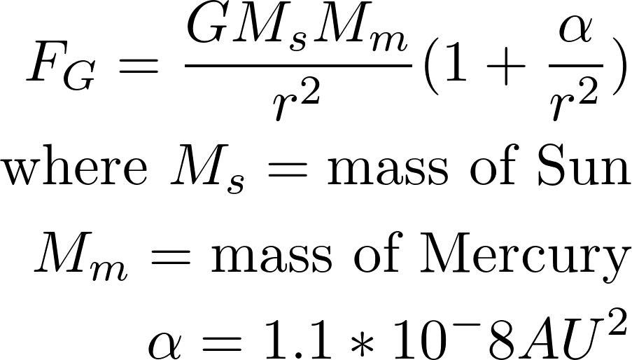
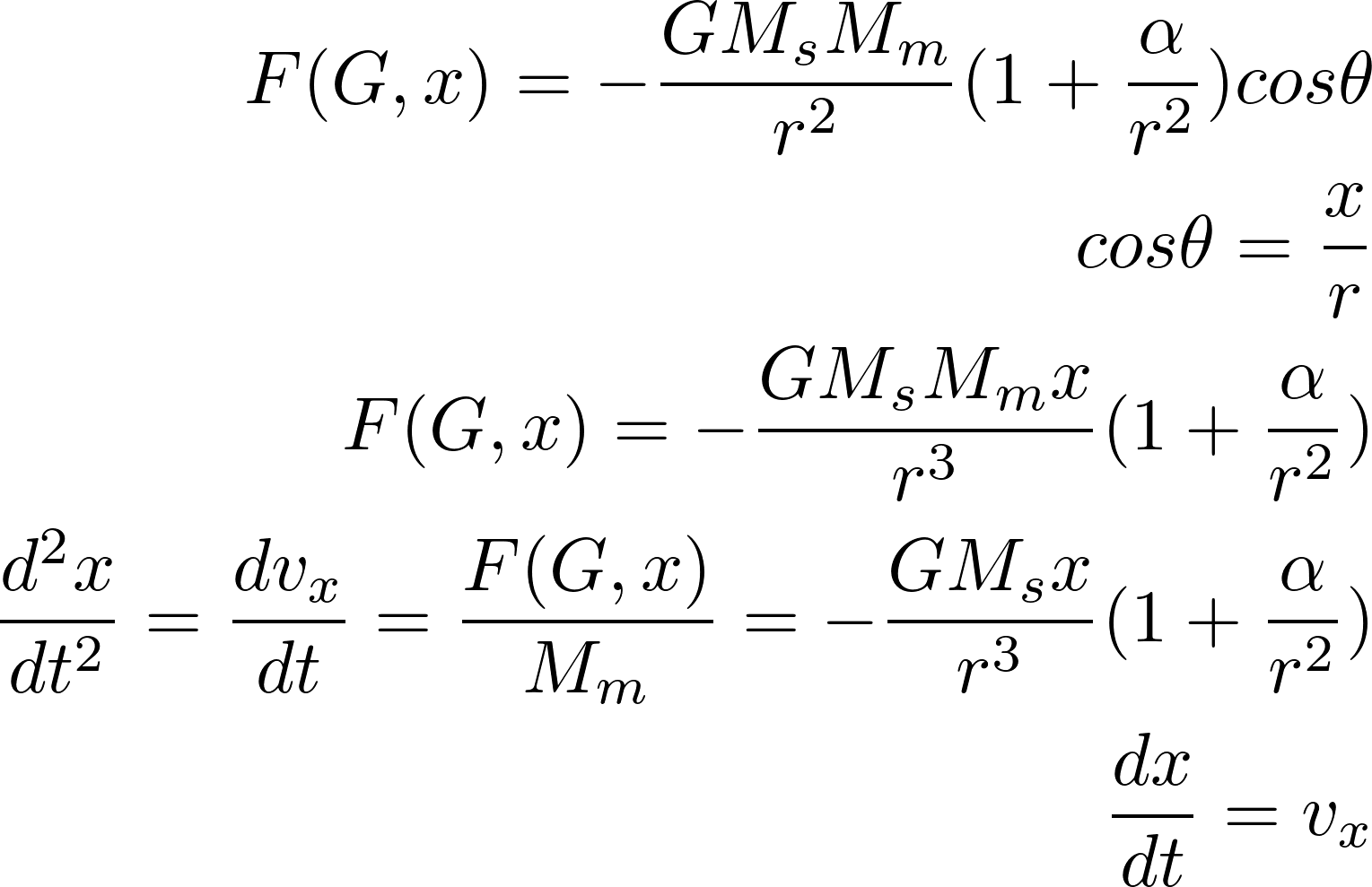
For centuries astronomies had a prediction of Mercury’s orbit from Kepler’s laws which measurably differed from observational values. What astronomers found was that Mercury mostly obeyed Newton’s inverse square law for its motion, but deviated because the orientation of the orbit’s axes was rotating over time. This is referred to as the precession of the perihelion, because the perihelion (the point in the orbit at which Mercury is closest to the Sun) lies along the semimajor axes. The source of the deviation from theory was a mystery until Albert Einstein released his paper on general relativity in 1915, in which he claimed his new theory explained the precession of the perihelion of Mercury due to the relativistic gravitational effects from the other planets (particularly Jupiter). Einstein’s adjustment to the inverse square force law is as follows:

The value for alpha shown above is the value calculated from general relativity; for this simulation, a much larger value of alpha is used so that the simulation doesn’t have to run as long to show precession. The value used in the main code of this program is .0008.

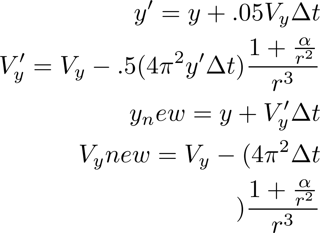
We then use the force law to calculate the velocity and position of Mercury. The derivation for the position and velocity with respect to x is as follows:

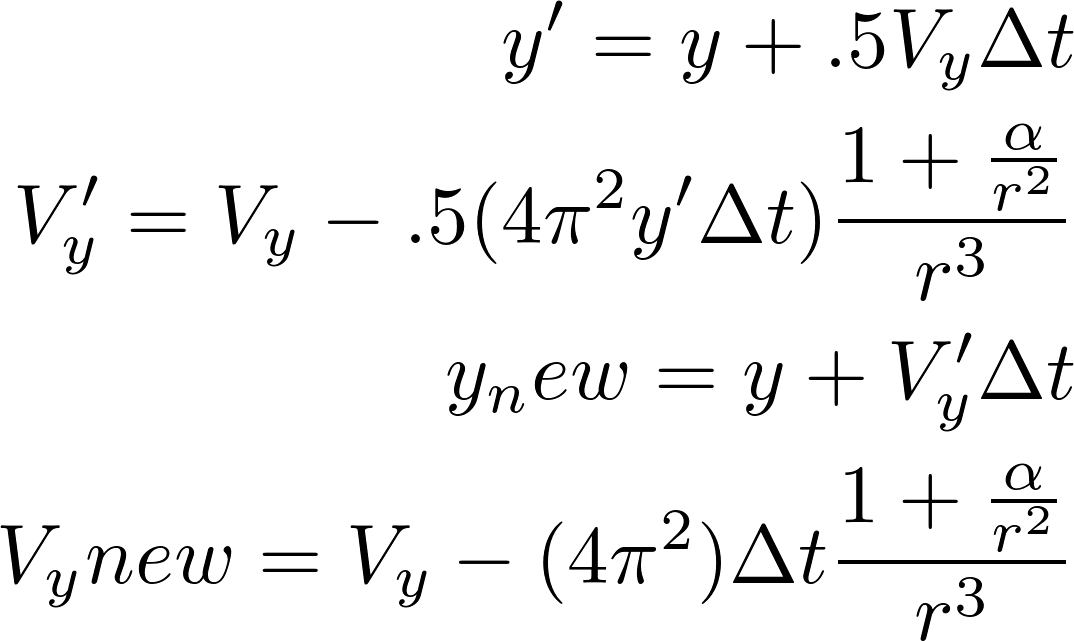
The derivation is virtually identical with respect to y. We then use these differential equations to create a computational algorithm; I chose to use the Runge-Kutta method because I felt that updating the values within the orbit computation loop would lead to a more accurate simulation.

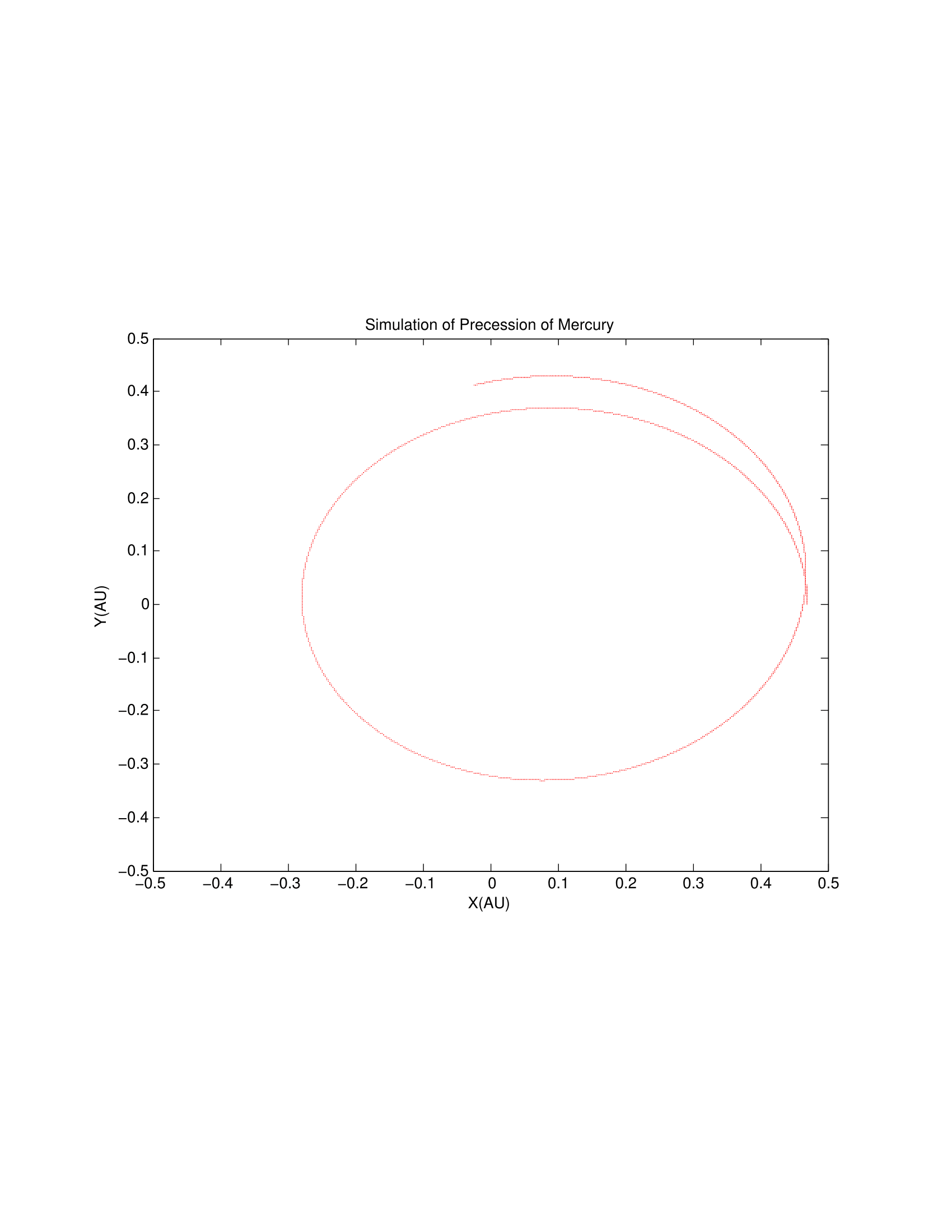
A representative graph is also included to show how the orbit changes over time.

Now that we have a code for the movement of Mercury, the next step is to find where the perihelions of each orbit lie. I did so by first conceptualizing what happens at the perihelions. Because the perihelions are the most rounded parts of Mercury’s orbit, the change in the distance from the Sun will be very small or slightly negative as Mercury moves closer to the Sun. Using this knowledge, I then find the position at these points and convert it to an angle. Angle is then graphed against time to show how the perihelion precesses over time.

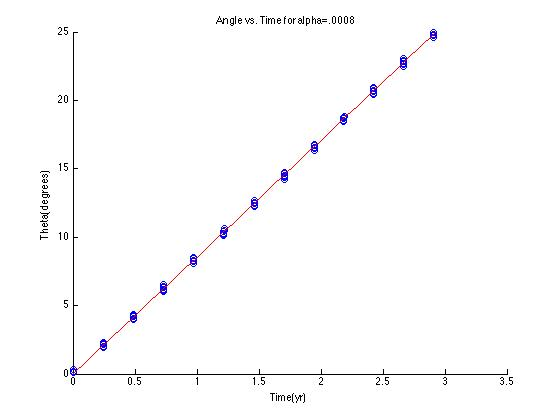
The goal of this graph is to find the fit slope of our angles so as to compare our computed precession rate to the analytical precession rate per unit alpha, 1.1 * 10^4 degrees per year per unit alpha. Using this value, we should be able to multiply it by the value of alpha predicted from general relativity to find a precession rate of about 1.2 * 10^4 degrees per year, or 43 arcseconds per century.

Continuing the program, I ran the precession simulation for values of alpha from .0001 to .004. I then created arrays to hold these alphas and their corresponding precession rates per alpha and plotted both with a fit line. The slope of this graph multiplied by alpha from general relativity is compared to the analytical values.

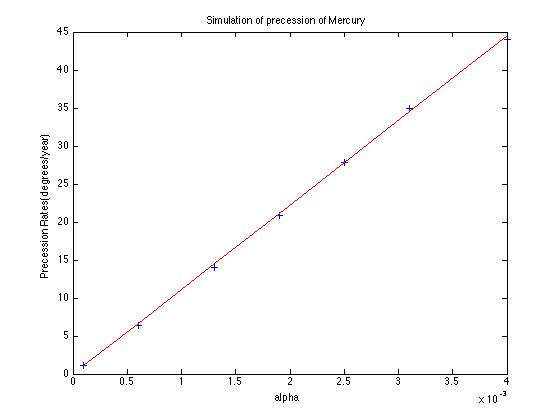
The slope calculated from the angle vs. time graph was 8.4516 with an r value of .749. Therefore the precession rate per alpha here, calculated by slope/alpha, is 1.067*10^4 degrees/year/unit alpha, which compared to the analytical value is a relative error of 2.9%. This precession rate per alpha is then calculated again in the slope of the second graph, which comes out to 1.1139*10^4 degrees/year/unit alpha, a relative error of 1.9%. Multiplying by Einstein’s alpha, we find a precession rate of 1.2253*10^-4 degrees/year or 44.11 arcseconds/century, with relative errors of 2.1% and 2.6% respectively.

Kirkwood Gaps

When astronomer Daniel Kirkwood plotted the number of known asteroids against their orbital radii, he found significant “gaps” of asteroids- orbital radii at which few or no asteroids were found to exist. Eventually he discovered that these orbital radii were in resonance with Jupiter, the largest planet and, as seen by the precession of the perihelion of Mercury, therefore the most likely to perturb the orbits of other objects in the solar system. This resonance is a ratio of the orbital periods for two objects rotating around the same central body of mass, and is related to the orbital radii of the object.  So in this example this project, the orbital period of an asteroid located at the 2/1 resonance point with Jupiter will be one half that of Jupiter’s, so it will complete two orbits for every one Jupiter completes. The relation between orbital period and orbital radii is given by Kepler’s Third Law:

where P is orbital period and a is orbital radius; this proportion holds for all objects orbiting the Sun. Knowing that Jupiter’s orbital radius is 5.2 AU, we can calculate the position of asteroids at resonance points by this ratio; i.e. at the 2/1 resonance, the orbital radius is 3.27 AU, 2.5 AU at the 3/1 point, and so on. We can also use the calculated radius to find the initial velocity by the equation for orbital speed:

The reason why Jupiter perturbs the asteroids so much at these radii is due to resonance- because the object in resonance is closest to Jupiter at the same several points in its orbit (for example, twice in the orbit of the 2/1 resonance), the perturbations from Jupiter will be largest only here and cause highly erratic orbits over time. The same phenomenon doesn’t happen at other radii because Jupiter’s perturbations occur at random points on the asteroid’s orbit and altogether cancel each other out over time.

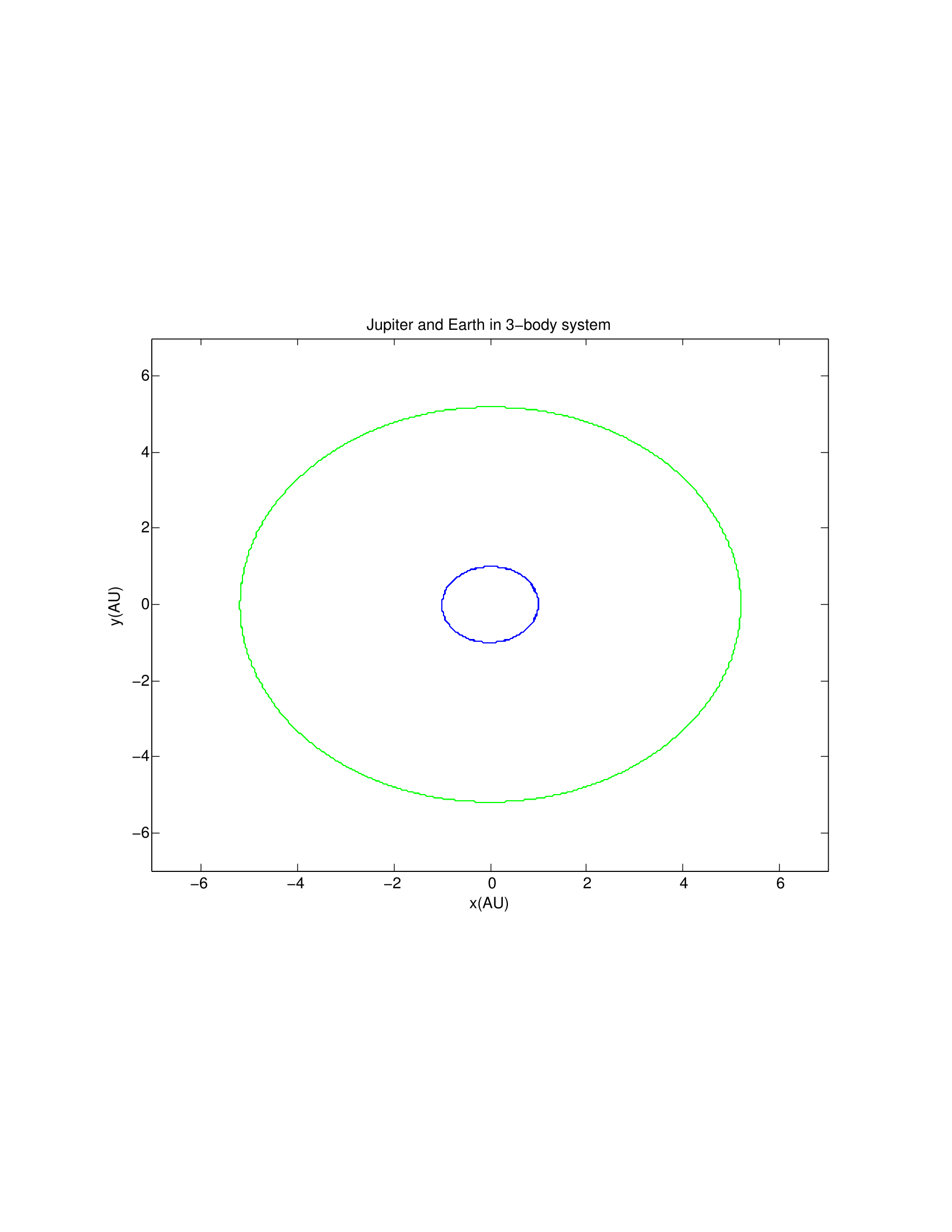
My code begins with the 3-body system as described on page 115 of Giordano and Nakanishi using the Euler-Cromer method. First I tested my code to demonstrate it worked without adding any asteroids:

Then I added asteroids at and around the 2/1 resonance point. Normally when adding more bodies to such a system, the new bodies interact with and change the orbits of the original objects, but because the mass of the asteroids is negligible as compared to all 3 objects already in the system (the Sun, Earth, and Jupiter), this effect can be ignored. The highly erratic 2/1 resonance is shown in blue:

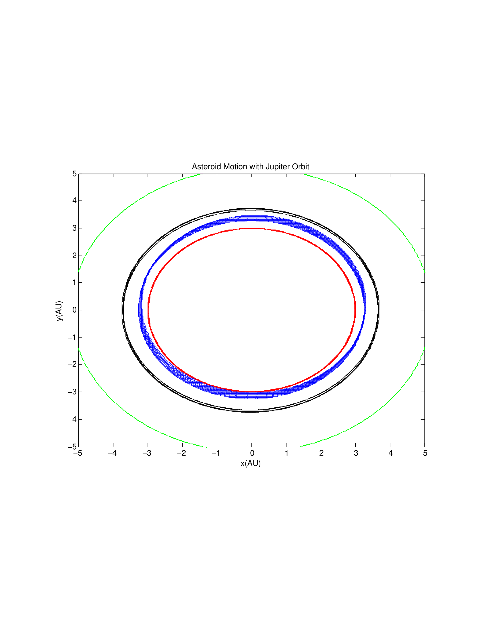
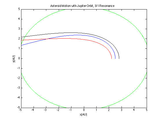
The other two asteroids demonstrate how little Jupiter perturbs their orbits. I then added asteroids at the 3/1, 7/3, and 5/2 resonance points, but found a very different effect:

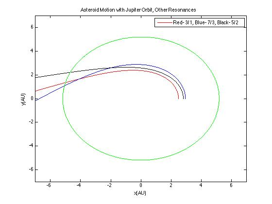
I originally thought that this was an error in the simulation, most likely caused by too many objects in the system, but I am now confident this is an accurate approximation of the involved physics; the explanation is in the following section.

Conclusion

Because the precession rate of Mercury has already been found analytically, it hardly comes as a surprise that the computational solution closely matches both theory and observation. The small relative errors compared to the analytical values shows the program is successful. While figuring out how to find the perihelion as it rotates was difficult, the rest of the program is straightforward because it follows from the known force equations. The program also demonstrates how known physical values can be altered to make computation easier, such as using a much larger alpha than in reality so as to speed up the calculation. While it might be more physically realistic to calculate the precession rate using a system with more massive bodies, at least including the largest perturber Jupiter, the calculated values are good enough to conclude the current simulation is sufficient in verisimilitude.

The program for the Kirkwood Gaps demonstrates how one very particular physical property, resonance, can have a very large effect when massive bodies are concerned. The first asteroid graph demonstrates this quite effectively, as the asteroid found in the 2/1 gap is perturbed much more than the outermost asteroid which is significantly closer to Jupiter. The graph of the other resonance points demonstrates exactly why it is that the Kirkwood gaps exist: eventually the perturbations from Jupiter become so large that the orbiting object is ejected entirely. The asteroid at the 2/1 resonance point isn’t ejected because it has the lowest frequency of interaction with Jupiter. At the other resonance points, Jupiter perturbs its orbit enough to eject it, because of the higher rate of encounter- the asteroid at the 3/1 resonance point is effected by Jupiter one more time than the 2/1 asteroid per orbit, a difference which has significant consequences over time. This program serves as a successful example of how a computational simulation can lead to greater understanding of the underlying physics even when an exact answer isn’t possible or even necessary. It is also worth noting that a phenomenon similar to Kirkwood gaps occurs with the rings of planets; for a real-life example, the rings of Saturn have gaps in them because the gaps are in resonance with one of Saturn’s moons.

Code:

https://drivenotepad.appspot.com/app?state=%7B%22ids%22:%5B%220B0gZLI_X8KZXWkxEbHVEVHlLbjQ%22%5D,%22action%22:%22open%22,%22userId%22:%22116986450796621489073%22%7D

https://drivenotepad.appspot.com/app?state=%7B%22ids%22:%5B%220B0gZLI_X8KZXSHNTaWlLQkhfZE0%22%5D,%22action%22:%22open%22,%22userId%22:%22116986450796621489073%22%7D

https://drivenotepad.appspot.com/app?state=%7B%22ids%22:%5B%220B0gZLI_X8KZXWlV3aDZFQThhaFk%22%5D,%22action%22:%22open%22,%22userId%22:%22116986450796621489073%22%7D

For the second week of this experiment I chose to begin my analysis by focusing in on a topic I believe I’ve glossed over thus far: orbital resonance. What I have neglected to mention is that this “resonance” is a ratio of the orbital periods for two objects rotating around the same central body of mass, and is related to the orbital radii of the object.  To start with an example relevant to this project, the orbital period of an asteroid located at the 2/1 resonance point with Jupiter will be one half that of Jupiter’s, so it will complete two orbits for every one Jupiter completes. The relation between orbital period and orbital radii is given by Kepler’s Third Law, that the ratio

where P is orbital period and a is orbital radius is a proportion that holds for any object rotating around the Sun. This was used to calculate the location of the 2/1 resonance at 3.27 AU, knowing the orbital radius of Jupiter to be 5.2 AU and the using a ratio of periods as 2:1 for Jupiter:asteroid. We also can use the equation for orbital speed to calculate initial velocity of an object at a certain orbital radii:

where G is the gravitational constant, M is the mass of the Sun, and r is the orbital radii. I used a value of 39.5 for G with time in years, distances in AU, and masses in solar masses for simplification; we already know the distance is AU, and the mass of the Sun in solar masses is, obviously, 1. This is very useful to this simulation, in terms of understanding that the initial values chosen in the system are not arbitrary; significant deviations could lead to the code breaking. It is also helpful to us for calculating the initial conditions for an asteroid at another radii in resonance with Jupiter, or a Kirkwood gap. This week I added asteroids around the 3/1 resonance radii. Using Kepler’s Law as stated before, this orbital radius was calculated to be about 2.5 AU (which matches the known value) for an initial orbital velocity of 3.97 AU/yr. I also placed two asteroids both closer and farther to the Sun for comparison. I am also including the orbital graphs for the 2/1 resonance from last week as comparison.

untitledrealam

For some reason, the orbits of the asteroids around the 3/1 resonance is even more irregular, perhaps caused by perturbations from planetary bodies other than Jupiter- namely, the Earth or the Sun. In the next week I will be analyzing what causes this stark change in orbit.

For my precession of the perihelion of Mercury program, I added the ability to calculate the position of the semi-major axes by surmising that on these axes not only will the perihelion lie, but the rate of change in radius will be small because the orbit becomes more elliptical, rounds out, and slows down. This assumption is based on Kepler’s Second law, that a line joining a planet and the Sun sweeps out equal areas during equal intervals of time; if the radius is largest here, it will be sweeping over more area, so the planet will move more slowly at these points. The position is then converted from Cartesian coordinates to polar coordinates. I then plot time against the position angle theta, take a linear fit through the data points, and take the slope to be the rate of precession. Afterwards, looping over an interval of alpha values, I will plot alpha against the precession rate, fit the data points, and take the slope to be the rate of precession. Unfortunately, when I tried to plot time against the angle theta, I kept receiving a value of close to 0 for the precession rate (slope). Without this slope, I am unable to calculate the precession rate for any values of alpha, and therefore cannot yet compare to the theoretical or expected value for the precession rate. I need to spend the next week debugging and figuring out how to make this program output the data I want it to. 

https://docs.google.com/document/d/1UBlg3d4G4RBf1pFgHE8AO1PzGjMjqwBs2hGTOAQ3FY4/

https://docs.google.com/document/d/1_GCUtQHpeSyNeQlUyF8ofSNFEFvcEyW8BAWswCMKjQ4/

The first simulation used in this project was for the precession of the perihelion of Mercury. This involves calculation of Mercury’s orbit using the force law as predicted by general relativity:

We can use the above equation to calculate position and velocity; I used a second-order Runge-Kutta Method. Equations shown are the same for x and y:

Once we have the proper position of Mercury we can convert said position to an angle theta. Then, plotting time against theta we can do a linear fit, the slope of which will be our desired rate of precession. A simulated orbit for Mercury, using alpha = .008, appears as shown:

which already shows the precession of the perihelion over time. In the upcoming weeks I need to more closely investigate the rate of this procession.

The second part of the project involves the investigation of Kirkwood Gaps, or the odd behaviour of solar satellites at certain orbital radii which “happen” to coincide with resonances of Jupiter’s orbit. This meant creating a multi-body simulation (I chose 3-body), so as to calculate the position and velocities of our planets (here, Earth and Jupiter), which are then used to calculate the position and velocities of our asteroids. Luckily, the mass of the asteroid is negligible as compared to that of our largest and most impactful orbiting body, Jupiter, and so the effect of the asteroids on Jupiter’s orbit can be ignored. The initial radius and velocity values used for the asteroids are found in Table 4.4 in Giordano and Nakanishi. Again the Runge-Kutta method was used to compute values. The equations used to calculate these values for planets are similar to the Runge-Kutta equations above and are shown by others doing similar celestial mechanics problems. Using this method I plotted first the orbits of Earth and Jupiter, to make sure my simulation worked:

and then plotted the asteroids’ orbits:

The blue orbit above is for the asteroid found around the 2/1 resonance orbit (ratio of axes is 2:1 for Jupiter:asteroid); here is a visual representation of the effect Jupiter can have on other objects, significantly disturbing their orbit. The next step in this program is to add complexity- more asteroids and a better graphical representation of where these orbital radii “gaps” occur.

Matlab Code:

https://docs.google.com/document/d/1hHy4D-B7eWIbknoHlLHJKvlyEtecRhIF7wupYeuFF1s/

https://docs.google.com/document/d/1jOSlib_gAtcADT_Mc0qFi2PA8n1I2nPnxqqOk_0f34w/

The goal of this project is to investigate two problems in celestial mechanics for which a computational solution is quite valuable: the precession of the perihelion of Mercury and Kirkwood gaps, both found in Chapter 4 of Computational Physics by Giordano and Nakanishi. In the case of Mercury, the precession can be calculated analytically thanks to general relativity, but a computational solution is easier to obtain. Giordano and Nakanishi describe the process of obtaining the rate of precession, keeping in mind that this variable must be adjusted for practical computation times (that is, not 230,000 years), using the force law predicted by general relativity:
F_G ≈ (G M_S M_M)/r^2 (1+a/r^2 ),
Where M_M≡mass of Mercury, M_S≡mass of Sun ,a ≈1.1 ×〖10〗^(-8) 〖AU〗^2.
Part of the project will be to compare different computational methods for analyzing this procession, particularly the Euler-Cromer method and Runge-Kutta (which uses the Euler-Cromer method to update its values). Using a two-body system simulation, the value for rate of procession can be found by varying until it matches expected, observed rates.

The second computational problem covered is one for which an analytical solution is difficult, as the system is considered chaotic. In our solar system there are certain “gaps” in orbital radii from the Sun at which there are far fewer asteroids. Numerically it can be found that these gaps occur at certain resonances with Jupiter’s orbit, such as 2/1, 5/2, 7/3, etc. Running a simulation to find Kirkwood gaps and investigate asteroids’ paths near these gaps first involves construction of a multi-body model, at least a two-body system for the Jupiter and Sun, and for more accuracy (if time permits) a three-body system along with the Earth. Luckily the magnitude comparison between Jupiter and an asteroid makes their mass insignificant, meaning their gravitational force can be excluded from the simulation without much effect on accuracy of the program. An analysis of the asteroid’s orbits will also naturally include a discussion of chaos, described in Chapter 3 of Giordano and Nakanishi.

Timeline:
Week 1: Continue background research on physics and computational methods of analysis, write code for precession of perihelion of Mercury, begin (and hopefully finish) writing code for 2- or 3-body system in Kirkwood problem
Week 2: Adjust solar system model to include simulations of asteroids, their paths/orbits, finish all code, begin gathering data.
Week 3: Finish gathering data, finish all research, comparison to actual observed/computer values from literature sources.
Week 4: Finish data analysis, write-up for project, prepare presentation.

Sources:
Computational Physics, Giordano and Nakanishi, Chapters 3 & 4.
Mercury’s Perihelion from Le Verrier to Einstein, N.T. Roseveare.
Chaotic Dynamics in the Solar System, J. Wisdom.

For my computational project I would like to investigate two particular topics in celestial mechanics: the precession of the perihelion of Mercury and Kirkwood gaps. Astronomy is a very precise science, but nevertheless deviations from the accepted laws exist, and sometimes the exact results are poorly known; in these situations computational answers are the most useful and feasible. One such deviation from the accepted laws (here, Kepler’s laws) is the precession, or the rotation of the orientation axes of its orbit, of the planet Mercury- that is, the point at which Mercury is closest to the Sun rotates moves, most likely due to the gravitational effect from the other planets. This precession can be calculated using computational methods. A similar situation arises with the asteroids that orbit in our solar system- something, most likely the gravity of other planets, is causing a deviation from known laws, only here, the asteroids are conspicuously absent from certain orbital radii. The gaps, mostly caused by Jupiter, are referred to as Kirkwood gaps and are found at particular orbital resonances with Jupiter (i.e. 2/1, 3/1, 5/2 resonances). The same process occurs with the rings around a planet such as Saturn- for some orbital radii there is no such ring. The occurrence of such gaps, in orbital location and at resonance point, can be found via computational methods.