Category Archives: Spring 2014

Conclusion: Corrections and Deconvolution

Update:

I concluded in my preliminary data post that the ‘Convolve’ function has its limitations and will not work properly with complicated functions. That may be so with relatively obscure functions, but I was wrong in my example. When I computed the convolution the long way by taking the Fourier transform of the product of Fourier transforms, I used the ‘FourierTransform’ function. I should have used the ‘InverseFourierTransform’ function instead. A Fourier transform of a Fourier transform is not necessarily the same as the inverse Fourier transform of a Fourier transform.

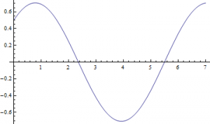
If f_1(x)=exp(-x)unitstep(x) \quad f_2(x)=cos(x), then through both methods I yield this plot:

Update

Mathematica file: https://vspace.vassar.edu/zerogoszinski/Update.nb

Vspace works better on Macs. If you are not using a Mac, please open the file from the Google Drive folder located at the end of this post. The file name is called ‘Update’.

Deconvolution:

Convolution has applications in imaging, in that a blurry image is simply the convolution of the image and a lens or instrumental function. This function is also called ‘point-spread function’ (PSF). Convoluting two functions is simple since the individual functions are known. Deconvolution is the reverse process, in which you have a convolution and you want to extract the desired image. This requires an understanding of the blurring function, which requires understanding the system that is causing the distortion. Extracting the pure image is much more difficult since every blurring variable needs to be taken into account. A perfect PSF is impossible to determine, so accounting for this function requires good approximations (4). Deconvolution is very important in astronomy, since all data comes from optical based systems. Even a perfect lens convolutes images, as they have unique diffraction patterns. The best focused spot for a camera lens is called the Airy disk:

\theta=1.22f\lambda/d

f is the focal length, \lambda is the wavelength, and d is the diameter of the lens.
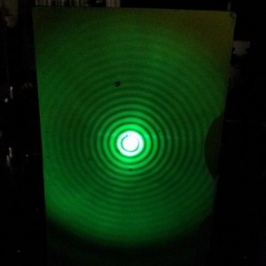
http://upload.wikimedia.org/wikipedia/commons/thumb/4/4b/Airy_disk_created_by_laser_beam_through_pinhole.jpg/480px-Airy_disk_created_by_laser_beam_through_pinhole.jpg

http://upload.wikimedia.org/wikipedia/commons/thumb/4/4b/Airy_disk_created_by_laser_beam_through_pinhole.jpg/480px-Airy_disk_created_by_laser_beam_through_pinhole.jpg


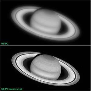
Here is an example of deconvolution in action:

http://opticalengineering.spiedigitallibrary.org/article.aspx?articleid=1183218

“Experience with the Hubble Space Telescope: 20 years of an archetype”
http://opticalengineering.spiedigitallibrary.org/article.aspx?articleid=1183218

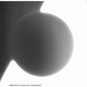
A particularly cool example of the effects of PSF in astronomy is the black-drop effect during the transit of Venus. The black-drop effect is an optical effect where the planet seems to stick to the edges of the star during ingress and pull apart like taffy as it enters the surface. Calculating the transit time would determine the orbital period of Venus. Kepler’s third law would then determine the radius of orbit. Astronomers of the 18th and 19th century wanted to figure this out in order to determine the actual size of the solar system. The black drop effect made it difficult to determine the exact moment Venus entered the Sun’s surface. The cause for this effect was discovered to be mostly due to PSF (Schneider, G., Pasachoff, J. M., Golub, L., 2004, Icarus, 168, 249). Poor optics creates this optical illusion, and accounting for point-spread function [and solar limb darkening] eliminates this effect.


Created by Zeeve Rogoszinski using data taken from Big Bear Solar Observatory.  http://imgur.com/p19moKI

Click to see the animation.
Created by Zeeve Rogoszinski using data taken from Big Bear Solar Observatory.
http://imgur.com/p19moKI

As you can see convolution and deconvolution have important applications in optics. Light beams get distorted as they pass through matter, and the scientist needs to be able to determine what exactly he or she is looking at. If I had the time I would have tried to deconvolute my convolution in the previous post, and try to extract one of the optical filters. I would have first assumed I knew what the second filter looked like, and try to work out the procedure from there. I would then assume I have no idea how the filters behave, and try to blindly deconvolute the filters. This would require looking into the theory behind deconvolution in a more rigorous manner.

Transit Paper:

http://web.williams.edu/Astronomy/eclipse/transits/Schneider_jmp_lg_Icarus2004.pdf

All of my data:

https://drive.google.com/folderview?id=0BxRRP3LUVuftVmFCcnNPMWFhU1k&usp=sharing

Share

Conclusion: Diffraction Patterns of C. elegans

I set out to model the diffraction patterns created by C. elegans nematodes using mathematica, specifically using the diversely useful mathematical tool of the Discrete Fourier Transform. The Transform is a quick way to find the diffraction patterns from Fraunhofer diffraction and interference (far-field diffraction). In simpler language, $\left| FT^{2} \right|$ produces the diffraction pattern, which is an analysis of the Electric field strength across the aperture, in this case, the image. The goal of this project was to produce a “library” of shapes and their corresponding diffraction patterns. However, there were many obstacles that made it necessary for me to do quite a bit of relevant research.
When I started, I did not know that the type of diffraction I was studying was Fraunhofer. Diffraction patterns are a result of the type of wave and the type of experimental setup. In this case, the light source, the aperture, and the screen were are far enough away to classify it as far-field. Mathematically, $L>>\frac{b^{2}}{\lambda}=\frac{area. of. aperture}{\lambda}$ . The fact that this is an example of Fraunhofer Diffraction makes it possible to apply the FT (on Mathematica) to yield the diffraction pattern.

I came in with some preliminary knowledge of what Fourier Transforms were in theory. In general, when applied, it changes a function’s variable dependence: $F(t) \leftrightarrow \Phi (v)$. I did quite a bit of research on the derivations of the transform and understood the matrix calculations necessary to do the transform “by hand” (see Project Plan).

To produce good-quality images, it was also necessary to do quite a bit of exploring in the Mathematica Documentation Center, becoming familiar with a variety of image manipulation commands. Those included: sharpening, brightening, finding the pixel count and dimensions, cropping, changing the color scheme to grayscale, partitioning and reassembling images manually based on the pixel dimensions, and more, depending on what degree of manipulation the image needed.
All in all, the images produced are not only pretty, but informative and now available for reference. Because it is mathematically impossible to go from the diffraction image to the shape, it is necessary to have some type of library, like the one I created, to go in that direction. (It is impossible to do it mathematically because when the Fourier Transform is applied, the phase information of the light is lost as the data is converted to the complex space.) Therefore, my “library” is useful because I have made it possible to guess the approximate shape and orientation of the worm from the diffraction pattern for some basic worm shapes. Another application for this analysis is that a compilation of several consecutive diffraction patterns shows the thrashing frequency of the worm. For example, if you took several pictures within a few seconds and found the diffraction patterns, the amount that the patterns change corresponds to the “thrashing frequency,” or the quantifiable amount that the worm wiggles.

If I were to continue this project, I would continue to build upon the library in the same manner, testing to see if different input image qualities would make a difference in the final product (if different pieces of the worms were fluorescing, if the worm was glowing a different color, etc). Finally, I would construct a real library (instead of this evolving blog site) that was easy to navigate, and generally more accessible for research.

Share

Conclusion- RLC Circuits

Overview

In this post, I will draw conclusions from my previous final data post about both RLC circuits that I have modeled.

RLC Circuit- No Voltage Source

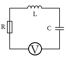
This RLC circuit [Figure 1] proved to be an interesting demonstration of the current in a circuit without a voltage source. The initial current running through the circuit is provided by the charged capacitor. However, this initial current undergoes damping due to the resistor in place, and the current running through the circuit pretty approaches zero pretty quickly.

1[Figure 1]

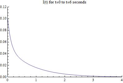
My model of this circuit verifies this idea since it shows an exponential decay of the current as a function of time [Figure 2]. After about 4 seconds, there is no longer an active current running through the circuit due to the resistor. My Mathematica notebook is easily set up for changing the values of the different components, and one can easily change them to see what effect this has on the circuit.

RLCCircuitsworking_finaldata1[Figure 2]

RLC Circuit- AC Voltage Source

The second RLC Circuit that I modeled was identical to the one above, except that it had an alternating current voltage source as well [Figure 3]. This allowed it to continue to have a current present despite the effects of the resistor.

circuitwithnumbers1[Figure 3]


Initially, I approximated the solution to the differential equation governing the circuit by ignoring the damping terms. This resulted in a an extremely good approximation, as the damping terms should only effect the circuit’s current flow in its first few seconds. After some computational hiccups that inaccurately displayed long-term variations in the current, I went on to graphically solve the complete form of the equation and graphed it to prove that the two damping terms only had a small effect in the first few seconds of the circuits behavior[Figure 4].

RLCCircuitsworking_finaldata9[Figure 4]

Final Remarks

Given the chance to work more on this project, I would develop manipulable animations within Mathematica that would allow one to change a given variable (ex. resistance, inductance, capacitance). This would allow the reader to easily see the effects that the different components have on the circuit. This would also be helpful from an educational standpoint as an applet to someone wanting to learn more about RLC circuits, or circuitry in general.

On a final note, I managed to learn a lot more about Mathematica and its differential equation solving capabilities. Solving the equations for these circuits by hand would have been an extremely length procedure, but once I provided Mathematica with the commands in the correct syntax, it solved them much faster than any human could. This project helped me appreciate the uses of computational tools in physics, and I am very glad that they exist.

Share

Final Data – E Fields of Spherical Objects

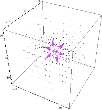
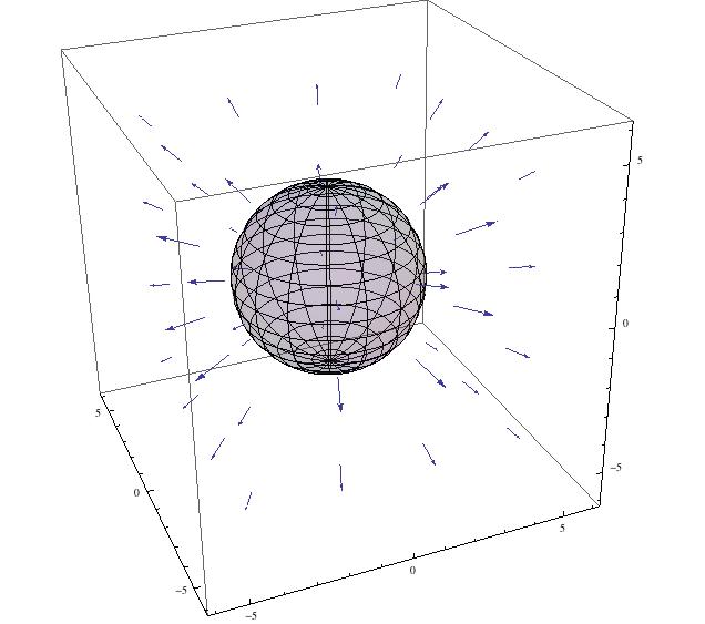
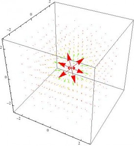
I began by modeling the electric field for a point charge +q, equal to the value of an elementary charge.

phys1


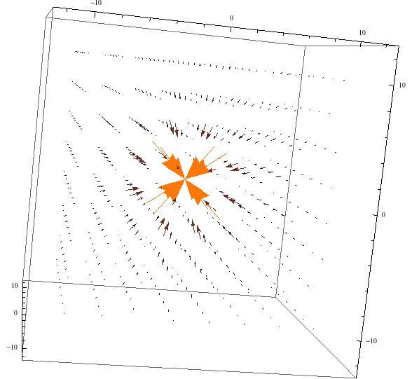
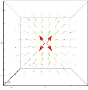
I also modeled the electric field of a point charge of -q.

phys2


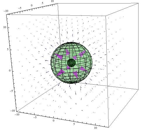
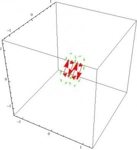
Next, I attempted to model the electric field due to spherical hollow conductor with total charge +q. First, I graphed a sphere of radius 5 using Mathematica’s SphericalPlot3D function. I superimposed the electric field of a positive point charge over this sphere, knowing that this would be incorrect. By Gauss’s Law, the stated configuration would result in an electric field of 0 inside of the spherical conductor, and an electric field following $\textbf{E} = \frac{1}{4 \pi \epsilon_0} \frac{q}{r^2} \mathbf{\hat{r}} $ for r > 5. The following image shows a partially transparent sphere with an electric field inside of it, violating Gauss’s Law.

phys3


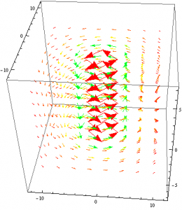
However, thanks to Brian Deer, I learned to use Mathematica’s RegionFunction, which allowed me to specify which regions of the graph on which the vector function would apply. The following now shows a hollow conductor of radius 3, with an electric field only present outside of it. Unfortunately, this step took a lot of time to work out, as I tried many different ideas to only get the field to show for certain radius values (i.e. be 0 inside of the conductor). I was unaware of RegionFunction, and even when I did learn what it was, I had trouble getting it to work with my model.

phys4


My updated Mathematica file can be found here.

Share

Final Results: Modeling Relativistic E&M

The next step of my project involved applying the modeling and manipulation code to different scenarios. In this case, I chose two scenarios that started as purely electric and developed magnetic components when considered in moving reference frames. The first was a continuous case- an infinite parallel-plate capacitor, and the second was a discrete case- a single point charge.

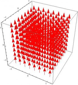
As has been well established, the field between two capacitor plates of charge density +/-σ is E=σ/2ε0. It is unsurprising then, that the E-field of a capacitor looks like this:

capacitor rest E

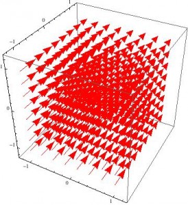
It is equally unsurprising that since there is no moving charge, there is no B-field. Then, when the system is considered in a reference frame moving at speed v relative to the capacitor and the transformation equations are applied, the following fields emerge for E…

capacitor rest E


and B…capacitor moving B

These look pretty dull, but are a few things to note about these figures. The first is that Mathematica is not able to show absolute magnitude of the vector fields: just the relative magnitude. That is, the arrows are the correct size relative to the other arrows in the box, but they are not necessarily to scale when compared to other fields. This is why the plots appear unchanged when v changes: the values of the vectors are all changing, but all at the same rate, so the pictures do not change.

The second notable feature is that (without accounting for the actual magnitudes of the fields), it is possible to see that even though the E- and B-fields both change, the direction of the net force does not. For a positive test charge at rest in the reference frame moving in the x-direction, it would experience only an electrostatic force in the z-direction in the rest case. For the moving case though, it would experience an E-field still in the z-direction and a B-field in the y-direction, both of which would result in a net force that is still in the z-direction.

Despite the simplicity of a point charge, this third case is actually the most interesting to look at because it is not infinite, but discrete. Thanks to every intro E&M course we’ve ever taken, we know that the E-field created by a test charge is E=q/r24πε0. The following vector plot or something similar probably appears in every intro textbook currently on the market.

pt charge rest E

Pretty boring, right? Completely spherically symmetric and falls off with r2 as expected. Now for the interesting ones: the fields in a moving reference frame. The E-field actually starts losing gaining so much of a y- and z-component that it appears to flatten out in the x-direction. The following figure is for v=0.75c

pt charge moving E

The B-field does something equally strange: it becomes somewhat cylindrical. However, in my code, this only appears at very high v (greater than 0.96c).

pt charge moving B

I get the feeling that if I could make mathematica show more detail, the field would not be in a perfect cylinder though. Since two rings of vectors appear on either side of the origin, it may be that the actual field has two lobes of some sort that are symmetric about the x-axis.

The last thing to note about this model is that when v=c, the simulation returns an error because it has to divide by zero when calculating gamma. Furthermore, the expression for gamma returns imaginary numbers for v>c, so this model is not useful for considering hypothetically how a system might behave if anything were able to move faster than the speed of light.

The mathematica worksheet associated with this can be found here.

Share

Final Data

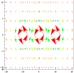
By using the formula for the magnetic field of a wire that I derived in my preliminary data,

(1)   \begin{equation*} \mathbf{B}(s) = \left\{ \begin{array}{lr} \frac{\mu_{0}I}{2\pi s}\widehat\theta & : s > a\\ 0 & : s < a \end{array} \right. \end{equation*}

I was able to model systems composed of current-carrying wires.

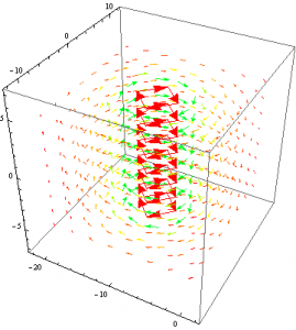
First I used the above equation and converted from Cylindrical to Cartesian coordinates. This was done because Mathematica will only plot vector fields in this form. I then plotted the resulting vector field due to a positive current.

1

This is exactly what we would expect to see for the magnetic field of current carrying wire as illustrated by the well known “Right-Hand-Rule”. The field lines are more intense towards the center of the of the wire while they decrease exponentially as they move further away. They are also oriented counter-clockwise since a positive current was used. Suppose now that we were to switch the current to a negative value.


2

As expected, the field lines behave in the same way as before expect they oriented in a clockwise fashion.

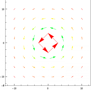
Below I changed the viewpoint of the magnetic field such that only the x,y plane is shown. This helps to visualize the field because the field does not change along the z-axis.


34

Now that I successfully found the Magnetic Field for a current-carrying-wire, I could make the system more complicated by adding additional wires.

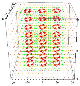
Suppose that some identical wires were placed parallel to each other at some distance.

.5


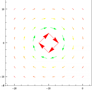
Again I changed the viewpoint such that only the x,y plane is seen. 6

As you can see in the above plots, the fields in between the wires have a certain type of symmetry. The field lines point in opposite directions and as they get closer to the midpoint between the to wires, they are of the same magnitude and cancel. It is safe to assume that as the distance between the wires approaches 0, the magnetic field between the wires will no longer exist.
Above and below the set of wires, the direction of the field lines due to each wire is the same: +x below the wire and -x above the wire. Coincidentally, this shares similar traits to the magnetic field due to a plane of current; the field lines above and below the plane will point either in the positive or negative x direction while there is no magnetic field anywhere along the plane itself. This shows that a plane of current can be viewed as a collection of parallel wires with no distance between them.

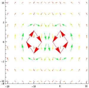
Suppose now that I had two wires parallel to each other but rather than having both wires having the same current, they are opposite to each other.


7 

If Mathematica were able to superimpose the magnetic fields from the different wires, I suspect that the resulting field would resemble that of a magnetic dipole. However, I have not been able to find a function that will do this given two different vector fields and am limited by time to model a magnetic dipole using an alternative method. Nevertheless, the field that I was able to model does share some similarities to that of a dipole. The symmetry of the field lines are the same as those of a dipole. This is a result of two equal and opposite currents.

Mathematica Notebook

References:

  • Griffiths’ Introduction to Electrodynamics 4th edition


Share

Final Data

My final data builds significantly from the preliminary data sets. In that set, I derived the equations for the electric field of a sphere, cylinder and the approximation of an electric dipole. Those were:

    \[ \textbf{E}  = \frac{q_e}{\epsilon_0 4 \pi r^2} \textbf{$\hat{r}$} \]

    \[ \textbf{E} = \frac{\rho R^2 }{2r\epsilon_0} \textbf{$\hat{r}$}  \]

Where the dipole was approximated as two point charges of opposite charge (i.e. two spheres of opposite charge).

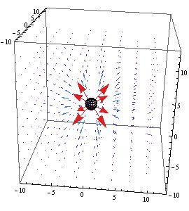
I went back to mathematica and overlaid a 3-D model of a small sphere on the previously plotted vector field of the electric field of a sphere, pictured below.

sfield

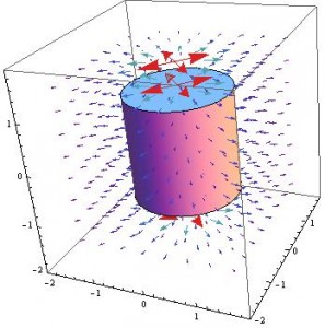
The same was done for a cylinder, both cases allowed for it to be seen how the geometries affected the electric fields.

cfield

For the electric dipole, an additional approach was taken to find the electric field. The equation for the electric potential of an “ideal” dipole is given as

    \[ V  = \frac{p_o \cos(\theta)}{\epsilon_0 4 \pi r^2} \]

For the purposes of simplification in Mathematica, the equation was re-written to absorb all the constants into one term:

    \[ V  = \frac{p \cos(\theta)}{r^2} \]

Now to find an expression for the electric field, use the formula:

    \[ \textbf{E} = -\nabla V \]

Which Mathematica can interpret and plot accordingly as:

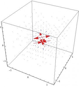
dipole

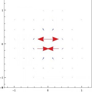
For a better view of how the vectors are interacting, look at this 2-D plot of the same field:

dipoleside

The code for the following models can be found here: Final Data

Share

Final Data- RLC Circuits

Overview

After talking with Professor Magnes after my preliminary results, I decided to first look at an RLC circuit with no voltage source, which is much simpler to model. Doing this allowed me to better understand the mechanism behind the circuitry and gain more experience with Mathematica as well.

After doing so, I returned to my progress with an RLC circuit with a voltage source and determined that the odd structural variations with the long-term structure were due to computational limitations of Mathematica (again, thanks to Professor Magnes for the suggestion). Since I had only developed the approximate solution, I went on to graphically solve for the full solution and see what the damping terms did to the solution.

Note: I included the findings from my preliminary data in this final data post (so it may seem redundant for a portion in the middle) since it was used in my final results as well. I figured it helps to have everything in one place for the reader.

RLC Circuit with no voltage source

Circuit Diagram and Mathematics

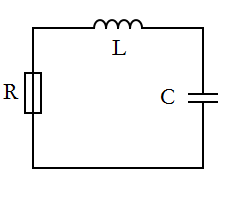
The first circuit we will examine is an RLC circuit with no voltage source. The initial potential difference is stored on the capacitor, but can not be recharged due to the lack of a voltage source. The three main components of this circuit are a resistor (R), an inductor (L), and a capacitor (C).

1[Figure 1]

The differential equation that governs this circuit is

LI''(t)+RI'(t)+\frac{1}{C}I(t)= 0 [1]

where L is the inductance, R is the resistance, C is the capacitance, I is the current through the circuit (which is the same at all places at one time since this is a series circuit), and t is the time.

Solving the Differential Equation

We can set arbitrary values for R, L, and C since they depend on the specific pieces of equipment themselves:

  • Inductance= 1 Henry
  • Resistance= 10 ohms
  • Capacitance= .1 farads

In Mathematica, the command to solve [1] looks like

\text{DSolve}\left[\frac{\text{Current}(t)}{\text{Capacitance}}+\text{Inductance} \text{Current}''(t)+\text{Resistance} \text{Current}'(t)=0,\text{Current}(t),t\right] [2]

which when solved, yields:

I(t)= c_1 e^{-8.87298 t}+c_2 e^{-1.12702 t} [3]

Completing the Full Solution via Graphical Solving

The two constants depend on the initial conditions of the circuit, which must satisfy Ohm’s Law of I=\frac{V}{R}. So, the initial current in the circuit must be 0.1 amps. Using a graphical guess-and-check method in Mathematica, I determined the value of the two constants to be approximately 0.05 each, resulting in a solution that is given by

I(t)= 0.05 e^{-8.87298 t}+0.05 e^{-1.12702 t} [4]

The plot of this equation gives us the current as a function of time, and looks like

RLCCircuitsworking_finaldata1[Figure 2]

This graph tells us that although the RLC circuit starts out with a current of 0.1 amps, it quickly dies down due to the lack of a voltage source and is not very interesting after a few seconds. Refer to the upcoming conclusion blog post for a bit more analysis.

Now, lets examine the RLC circuit with a voltage source (much more interesting!)

RLC Circuit with AC voltage source

Circuit Diagram and Mathematics

Now we can model an RLC circuit that consists of a capacitor, voltage source, resistor, and an inductor. To easily visualize this, I have constructed a basic circuit diagram (Figure 3).

circuitwithnumbers1(Figure 3)

The differential equation that governs this RLC circuit is given by

LI''(t)+RI'(t)+\frac{1}{C}I(t)= E_{0} \omega cos(\omega t) [5]

where L is the inductance, R is the resistance, C is the capacitance, I is the current, \omega is the resonant angular frequency,  E_{0} is an initial value dependent on the voltage source, and t is the time. The inductance (L), resistance (R), and capacitance (C)are all determined by their respective circuit components, which are easily changed out for different ones. \omega depends on the inductance and capacitance, and its value is given by

\omega =\frac{1}{\sqrt{LC}} [6]

What we have left in terms of variables are current (I) and time (t). For our purposes, time is the independent variable, which leaves the current in the circuit at any time to be the dependent variable. Now that we have established this, we can solve our differential equation [5] for current as a function of time (I(t)).

Solving the Differential Equation

In order to solve [5], I will use the equation solving powers of Mathematica. In particular, the DSolve function is used.  When plugged into Mathematica, the input line looks like:

\text{DSolve}\left[\frac{\text{Current}(t)}{\text{Capacitance}}+\text{Inductance} \text{Current}''(t)+\text{Resistance} \text{Current}'(t)=E_{0} \omega \cos (\omega t),\text{Current}(t),t\right] [7]

We must set values for resistance, inductance, capacitance, and  E_{0}. For this solution, I chose the same values as the first circuit :

  • Inductance= 1 Henry
  • Resistance= 10 ohms
  • Capacitance= .1 farads
  •  E_{0}= 1 Volt

When the command is run with the above values set, Mathematica generates the general solution, which is:

I(t)=c_1 e^{-8.87298 t}+c_2 e^{-1.12702 t}+0.040824(-Cos(3.162t)+e^{6.661*10^-16t}Cos(3.162t)-0.3564Sin(3.162t)+2.806e^{6.661*10^-16t}Sin(3.162t)) [8]

First, lets make sure that this solution is reasonable. The known form of the solution to the equation for such a circuit is given by:

I(t)=c_1 e^{r_{1}t}+c_2 e^{r_{2}t}+Asin(\omega t-\varphi ) [9]

The form of our equation [8] seems to match up pretty nicely with this known solution [9]. Now, lets examine [8] in more detail.

Our solution [8] looks a little daunting, but we can break it down into its components. The first two terms have constants that depend on the initial current running through the system, i.e. when I(t)=I(0). However, we can approximate the equation by only looking at the last term, which is a superposition of sin and cosine functions along with a couple exponential terms thrown in. The reason that we can apply this approximation is that the first two terms “damp out” quickly, and thus have exponentially less of an effect as time progresses. The reader may still be curious to see how much of an effect these terms have on the current flowing through the system: to that I say don’t worry! After my initial approximation, I will solve for these constants and compare the two cases.

Approximate Solution and Graphs

For now, we will deal with the approximate solution, which is:

I(t)=0.040824(-Cos(3.162t)+e^{6.661*10^-16t}Cos(3.162t)-0.3564Sin(3.162t)+2.806e^{6.661*10^-16t}Sin(3.162t)) [10]

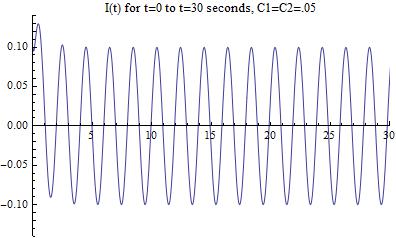
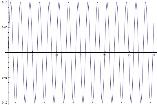
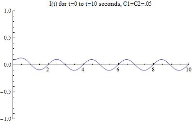
Now that we have this equation, we can use Mathematica to give us an idea of what the changing current looks like over a longer period of time. Figure 2 shows the current in the circuit as a function of time (I(t)) plotted over a 30-second interval.

30secondplot(Figure 4)

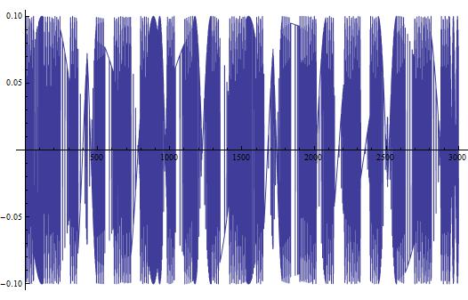
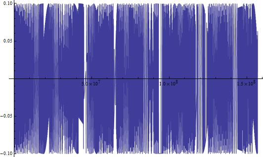
This looks like something we would expect! A sinusoidal wave that describes the changing current over time, just like our equations dictate. But, this is a short time-scale. What happens when we look at the changing current over a longer period of time? In Figure 3, I show the changing current over a longer time period (3000 seconds/50 minutes). In Figure 4, I repeat the process, but with the timescale being 5 years.

50minuteplot(Figure 5)

5yearplot(Figure 6)

In both Figures 5 and 6, we see some very interesting long-term variations in the current. Why does this occur?

Computational Limits

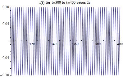
It is clear that Mathematica is displaying some odd variations that do not seem to have a set pattern. To investigate this and determine its cause, lets look closer at a range of time where the current seems to be irregular in the previous two figures. Specifically, lets look at the time scale between 300 and 400 seconds because it seems to have very strange behavior.

RLCCircuitsworking_finaldata1[Figure 7]

Looking at the graph above, we see that it looks completely normal! There are no strange variations and the current continues the predicted sinusoidal trend. This leads me to the conclusion that Mathematica has limitations that caused the irregular variations that we saw before, and that they do not actually exist in the data/circuit.

Completing the Full Solution via Graphical Solving

The next and final step in completing our model is accounting for the two initial terms that we left out. Lets take another look at the full equation.

I(t)=c_1 e^{-8.87298 t}+c_2 e^{-1.12702 t}+0.040824(-Cos(3.162t)+e^{6.661*10^-16t}Cos(3.162t)-0.3564Sin(3.162t)+2.806e^{6.661*10^-16t}Sin(3.162t)) [11]

We can see that they are exponential functions with a separate constant for each term. Solving for these constants quantitatively can prove to be difficult, so I will attempt to solve for them via a guess-and-check method using plots in Mathematica. I need to match the initial condition so that Ohm’s law is satisfied. So, I=\frac{V}{R} must hold in the initial state. This means that the initial current must be 0.1 amps. Lets try a few values for C[1] and C[2] and figure out graphically what they should be.

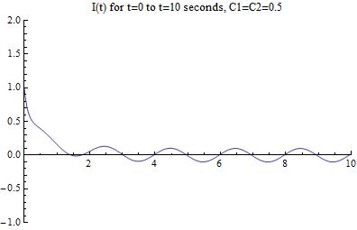
First, lets try values of 0.5 for each, resulting in the following equation:

I(t)=0.5e^{-8.87298 t}+0.5e^{-1.12702 t}+0.040824(-Cos(3.162t)+e^{6.661*10^-16t}Cos(3.162t)-0.3564Sin(3.162t)+2.806e^{6.661*10^-16t}Sin(3.162t)) [12]

The graph resulting from this equation is:

RLCCircuitsworking_finaldata6[Figure 8]

We can see that the initial current that this combination of constants is too high! It gives 1.0 amps, when we are looking for 0.1 amps.

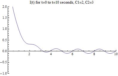
Lets try slightly higher values for each, as well as having different values for the two. The equation that results is:

I(t)=2e^{-8.87298 t}+3e^{-1.12702 t}+0.040824(-Cos(3.162t)+e^{6.661*10^-16t}Cos(3.162t)-0.3564Sin(3.162t)+2.806e^{6.661*10^-16t}Sin(3.162t)) [13]

Which produces the following graph:

RLCCircuitsworking_finaldata7[Figure 9]

Looks like we have gone the wrong way with our guess! Lets try lowering both the constants to arrive at the correct graphical solution (in reality, this took me many more iterations of guessing and checking):

I(t)=0.05e^{-8.87298 t}+0.05e^{-1.12702 t}+0.040824(-Cos(3.162t)+e^{6.661*10^-16t}Cos(3.162t)-0.3564Sin(3.162t)+2.806e^{6.661*10^-16t}Sin(3.162t)) [14]

Which results in the following graph:

RLCCircuitsworking_finaldata8[Figure 10]

The Graphical Solution

Now that we have arrived at the correct graphical solution, lets change the scaling of the graph to better match that of [Figure 2], which was the initial approximation that did not take into account the two damping exponential terms.

RLCCircuitsworking_finaldata9[Figure 11]


My conclusion from this final data will follow in my next blog post.


Resources

1. Circuit Diagram Maker- http://www.circuit-diagram.org/

2. The RLC Circuit- University of British Columbia-  http://www.math.ubc.ca/~feldman/m121/RLC.pdf

3. Mathematica Cookbook by Sal Mangano

4. Electronic Circuit Analysis for Scientists by James A. McCray and Thomas A. Cahill

5. Dynamical Systems with Applications using Mathematica by Stephen Lynch

6. Class Notes- Mathematics 228 (Methods of Applied Mathematics) taught by Matthew Miller


Mathematica Notebook

https://drive.google.com/file/d/0B3mtB6CQNnpjbXROcHl0VURzYlE/edit?usp=sharing

Share

Final Results: Convolving Optical Filters

Optical Filters

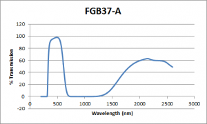
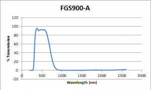
Now that we have the theory down, let’s apply convolution to actual data. The model here is two optical filters placed on top of each other. The light beam will go through both filters, and come out the other side somewhat convoluted. I have chosen two optical filters from thorlabs:

  • Item #FGB37-A: BG40 Colored Glass Filter, AR-Coated: 350 – 700 nm
  • Item#FGS900-A: KG3 Colored Glass Filter, AR-Coated: 350 – 700 nm

The plots of their transmission percentage as a function of wavelength are shown below:

FGB37A FGS900A

Notice the first plot down does not tend to zero as the wavelength increases. My hypothetical light beam will have a wavelength of around 500 nm, so I cropped out the two peaks from each plot from 200 nm to 1000 nm. I also added 200 zeroes to each end extending my plots from 0 to 1200 nm. I did this so that the transformations would have as little noise as possible.

Convoluting the two functions requires using the exact same method described earlier, but instead using discrete Fourier transformation. My first attempt at convoluting these two plots failed. The convolution gave me complex solutions, and I need my solutions to be real. I tested the method on two Gaussian functions by extracting artificial data points through the function ‘Table’. The list of data presented was not in the same format as the imported optical filter data. Mathematica does not like Excel, and the data imported was in the format of a list of 1×1 matrices of each point [The data also needed to be one dimensional, so the x-axis represents data point number. Fortunately the amount of data points is equivalent to the range of wavelengths, so for all intents and purposes the x-axis represents wavelength]. To bypass this confusion I saved my data as a text file and imported the list as a list. For example:

a = Import[“C:\\Users\\Zeeve\\Desktop\\EM Project\\FGB37-A test.txt”, “List”]

The data is now real. It should also be noted that the default setting for the Fourier transform is not the convention for data analysis. This requires using the tool FourierParameter to change the range from {0,1} to {-1,1}.

Capture


This is what my data looks like:

first attempt


The y-axis is the transmission percentage, and the x-axis is the wavelength.

Notice the peak is around 1000 nm. It turns out that the inverse discrete Fourier transform of the product of two Fourier transforms of data is not the convolution of the data. It is actually the cyclic convolution of the two data sets. If you go back to the original definition, one of the functions in the integral of the convolution is shifted by some value x’.

f_{1}(x)\ast f_{2}(x)=\int_{-\infty }^{\infty }\!f_{1}(x')f_{2}(x-x')\mathrm{d}x'

Notice also the y-axis and how it extends to beyond 5000. This is because my normalization constant was wrong. The square root of 2 Pi in the convolution algorithm is a normalization constant for Gaussian functions. Correcting this was simple. I used the ‘Normalize’ function to normalize my Fourier transforms, and used the product of those results:

v = Normalize[m]*Normalize[n] instead of c=Sqrt[2 Pi] m*n

Correcting the former issue is trickier. I need to cycle the function back to peak at around the 500 mark. I admit I am not familiar with the mathematically correct method of correcting this error, so I ball-parked it. The peak needs to be around 500 nm since the original data peaked at around 500 nm. Cycling the curve backwards required outside help. I used the method described in the first answer here: http://mathematica.stackexchange.com/questions/33574/whats-the-correct-way-to-shift-zero-frequency-to-the-center-of-a-fourier-transf .

The method uses the function ‘RotateRight’ to cycle a range of data a certain amount of points. My range of points extends from 0 to 1200, and I cycled 400 points. Now I have a plot where the x-axis is pretty much the correct wavelength for its corresponding value (although the values are off by a factor of 100, which is fine since it is simply a normalization correction), which is the convolution of the two optical filters:

convolution optical


Again here the y-axis is the transmission percentage, and the x-axis is the wavelength. The y-axis is off by a scaling factor.

For a complete transcript of the convolution, please check out the Mathematica script:

https://vspace.vassar.edu/zerogoszinski/Optical%20Filters.nb

Here are the text files:

https://vspace.vassar.edu/zerogoszinski/FGS900-A%20test.txt

https://vspace.vassar.edu/zerogoszinski/FGB37-A%20test.txt

Future:

For my conclusion I will discuss about deconvolution and some expansions on convolution.

Note: If the files do not work for you, I have uploaded all of my files to Google Drive which can be accessed in the conclusion. The concerning files are the Mathematica script ‘Optical Filters’, and the two text files ‘FGS900-A test’ and ‘FGB37-A test’. 


Share

Final Data and Conclusion

NOTE: some of the equations are too long to render fully. To see them in their entirety, either open the image in a new window or see the mathematica file

Force on the slug

In the preliminary data, an equation for the force in a railgun was calculated assuming a constant current in the system. This was:

    \[ \text{Fmag}(i,L,W)=\frac{\mu _0 \left(i^2 L \left(-L \sqrt{L^2+W^2}+L^2+W^2\right)\right)}{\pi  \sqrt{L^2+W^2}} \]

Where J is substituted for the I, because mathematica will not accept I for some strange reason. However, this is entirely inaccurate and essentially useless, as the current is almost never constant in time for a railgun. The graph does show, however, that for very small values of L, the force is small. This means that the slug must move into the loop far enough to experience a force before the current dissipates. Happily however, from the equation for the force calculated earlier, we can now find the total force on the system as a function of time using the equation of total current as calculated by Elias Kim.

    \[ \text{Fmag}=\frac{\mu _0 \left(L \left(-L \sqrt{L^2+W^2}+L^2+W^2\right)\right) \left(\frac{A Q_0 e^{-\frac{A t}{C \rho  (2 L+2 W)}}}{\text{C$\rho $} (2 L+2 W)}\right){}^2}{\pi  \sqrt{L^2+W^2} \left(\frac{A \mu _0 v \left((-\ln ) \left(L \sqrt{a^2+L^2}+L^2\right)+L \ln  \left(\sqrt{(W-a)^2+L^2}+L\right)-\ln  \left(L \sqrt{(W-a)^2+L^2}+L^2\right)+\ln  \left(L \sqrt{a+L^2}+L^2\right)\right)}{4 \pi  \rho  (2 L+2 W)}+1\right){}^2} \]

Where L is the instantaneous length of the loop along the rails, W is the rail separation (center to center), a is the radius of the rails, A is the cross sectional area of the rails, Qo is the initial charge in the capacitor, rho is the resistivity of the rails, v is the velocity, and C is the capacitance of the capacitor. We will then use this derived equation to solve for the force in two theoretical examples and provide simulations of the force as functions of time for each. For a small railgun, where a=.009, W=.03, C=450*10^-5 and Subscript[Q, 0]=1.8 we get

    \[ F=\frac{4 \left(\left(L \left(L^2-\sqrt{L^2+0.0009} L+0.0009\right)\right) \left(\frac{1.8 e^{-\frac{t}{(10 L+0.15) \rho }}}{(10 L+0.15) \rho }\right)^2\right)}{10^7 \left(\sqrt{L^2+0.0009} \left(\frac{9.04 k v}{10^{11} ((2 L+0.06) \rho )}+1\right)^2\right)} \]

However, although this is still more accurate than before, it is still not a completely accurate measure, as t and L are still expressed independently from one another. however, this issue may not be resolved as the equations of motion are too complicated to attain precise equations of motion.

For the military railgun, however, the force is significantly greater, with a C=1.5 farads, Qo=10000, W=.8, and A=.01 additionally, the logarithmic terms were solved for to be inside of a range of values, which were then plotted as the variable k. Additionally, it should be noted that the values of the capacitance and charge are derived assuming a 100% conversion between energy stored in a capacitor and kinetic energy. The resistivity was plotted to be at a minimum that of Aluminum.

    \[ F=\frac{4 \left(\left(L \left(L^2-\sqrt{L^2+0.064} L+0.064\right)\right) \left(\frac{10000 e^{-\frac{t}{(75 L+60) \rho }}}{(75 L+60) \rho }\right)^2\right)}{10^7 \left(\sqrt{L^2+0.064} \left(\frac{4 k v}{10^9 ((2 L+1.6) \rho )}+1\right)^2\right)} \]

These measures of force are significantly more accurate than the theoretical version shown earlier in the data. The reason for this is that aside from the previous issue of L and t still being unrelated, this graph demonstrates the correct behavior for this system. We can manipulate the values of L however, and can see a clear trend in the force as a function of time in the above manipulation. Upon firing, the force quickly reaches a maximum as both the loop becomes large enough and the current still is present in sufficient quantity to provide efficient acceleration, however, as time goes and the loop size becomes larger, this term then collapses to be insignificant. That being said, it is clear that even a small system can accelerate objects to incredible velocity. Additionally, the resistance in the circuit must be accounted for as it has a tremendous impact on the graph of the force.

By combining and altering our manipulations of the equations given above, a clear trend in the force appears. Most likely, the force will resemble an overdamped wave, as seen in classical oscillations and EM waves. This means the force will reach a maximum, then exponentially decrease until the slug leaves the rails.

Finally, by analyzing these examples and the general equations of force it is clear that there is an ideal set of dimensions for a given system to maximize the force upon the slug. If each value falls outside the ideal range, the force will quickly decline by several magnitudes from the maximum possible force.

The Inductance Gradient

Remember the force can also be given as

    \[ F=\frac{1}{2} i L_1 t^2 \]

The other way to measure the force experienced by the slug in a railgun is using the inductance gradient, L’, for the railgun, by which you can find the optimal measures for a given system. The inductance gradient is measured in microhenries per meter, accounting for the Mu term of the force. For most cases, this value is calculated experimentally, however, for a miniscale railgun, the method of Lagrangian optimization. The object of this method is to minimize the value of the goal function,

    \[ \pmb{P=G+\sum _{i=1}^m \lambda _i\left(J_{\max }(h,w,z)_i-J_{\text{material}}\right)}\ \]

The minimum of G is also proven to be the point of inflection in the P function. found using the second, series term of the P function. Eventually, this will form a regression, which can be evaluated using a system of equations to find the most efficient rail dimensions for a given system.

Where Jmax] is the maximum tolerable current density in the rails, and Lambda is an aribitrary constant. The Jmateral value is derived from the maximum tolerable current density of a copper cable (it comes from the material used in the system). The h, z and w, values are the dimensions of the rails. Jmax] is different from Jmaterial] because the current, attempting to take the shortest path through the system, will cluster in the corners between the rails and the slug.

Energy in a railgun

The most effective means to approximate the energy in the railgun is to use the capacitance and charge in the capacitor bank. Although this is extremely inaccurate while measuring the actual velocity and energy of the slug following firing of the system, it is an effective means to calculate the various constants going into the force. The muzzle energy can be calculated by measuring the kinetic energy of the slug following its expulsion from the loop, from this, it is possible to calculate the fraction of energy lost thermodynamically and frictionally in the system as discussed in the preliminary data. The energy in a capacitor is defined as:

    \[ W=\frac{Q^2}{2 C}=\frac{\text{CV}^2}{2} \]

The kinetic energy of any object is defined classically as:

    \[ T=\frac{\text{mv}^2}{2} \]

Using this we can theoretically calculate the efficiency of both our large and small railgun systems. For the small system, where 10 400V, 450 microfarad capacitors are wired in parallel, C=4500 microfarads, V=4000 V, the mass is 3.6 grams and the muzzle velocity was around 700 m/s. This gives the following values:

    \[ W=\frac{\left(4\ 10^3\right)^2 4500}{10^6 2}=3.6 \text{kJ} \]

    \[ T=\frac{0.0036 700^2}{2}=882 J \]

    \[ \frac{T}{W}=0.245 \]

For the small scale design, the system achieved a 25% efficiency in the transfer of energy. Although this appears to be a low efficiency, a standard firearm usually has an efficiency between 20-40%, and this is an extremely inefficient design for a railgun. The military, in their system tested in 2013, for which we modeled the forces earlier, the  kinetic energy was given to be 33MJ however, due to the fact that the precise specifications of the capacitors are classified, we cannot effectively measure the efficiency of the system. Their efficiency is most likely higher, probably around 60%. The reason for this is that for high efficiency designs, the slug design and rail geometry changes significantly. We have modeled the military design as a square barreled launch system, with rails on either horizontal side. However, it is likely that the real geometry is different, to increase the efficiency of the discharge, as well as reduce the inevitable wear caused by heat. Additionally, rather than routing the current through the slug, through a gap all the while dealing with high resistances and thermodynamic loss, the millitary system insulates the main body of the slug, while adding a material at the rear which when subjected to the initial current shock will become a plasma. This is a much more efficient design, and that, along with the ability to make the slug more aerodynamically efficient will increase the total efficiency of the system. Although we do not have the tools to fully explain the resistivity of the plasma (plasma physics is a graduate level study), the Spitzer resitivity of a plasma is given as:

    \[ \eta =\frac{\Lambda  \sqrt{m} \text{$\pi $Ze}^2 \ln }{\left(4 \pi \epsilon _0\right){}^2 \sqrt[3]{T k_b}} \]

*from http://silas.psfc.mit.edu/introplasma/ and Wikipedia, common knowledge to people who have taken plasma physics

Where Eta is the Spitzer resistivity, Z is ionization of nuclei, m is the electron mass, Curly Epsilon is the resistivity of free space, ln (Capital Lambda) is the Coulomb logarithm, k is Boltzmann’s constant and T is the temperature in kelvins. This value is presumed to significantly increase the efficiency. Additionally, the use of a plasma allows the system to be launched from rest, which as shown in the force approximations, significantly increases the efficiency of the system.

Acceleration on the slug

Using the derived equations of force found earlier, it is fairly simple to calculate the accelerations as functions of time in a railgun. Prior to showing, it ought to be noted that although the accelerations for even a small scale model are enormous, predicting in the hundreds of thousands, even tens of millions of metres per second squared, the slug only remains in the rails for periods best measured by microseconds, and the force dissipates even faster.

Given this understanding, the general form of the acceleration can be written as:

    \[ \text{Amag}=\frac{\mu _0 \left(L \left(-L \sqrt{L^2+W^2}+L^2+W^2\right)\right) \left(\frac{A Q_0 e^{-\frac{A t}{C \rho  (2 L+2 W)}}}{\text{C$\rho $} (2 L+2 W)}\right){}^2}{m \left(\pi  \sqrt{L^2+W^2} \left(\frac{A \mu _0 v \left((-\ln ) \left(L \sqrt{a^2+L^2}+L^2\right)+L \ln  \left(\sqrt{(W-a)^2+L^2}+L\right)-\ln  \left(L \sqrt{(W-a)^2+L^2}+L^2\right)+\ln  \left(L \sqrt{a+L^2}+L^2\right)\right)}{4 \pi  \rho  (2 L+2 W)}+1\right){}^2\right)} \]

For our two examples, the smaller scale measure using a projectile weighing 3.6 grams and our large scale millitary model used a projectile mass of 3.2 kg. Subbing those in and generating manipulations, we arrive at:

    \[ \pmb{a=4*10^{-7}\frac{\left(L \left(.0009+L^2-L\sqrt{.0009+L^2}\right)\right)\left(\left(\frac{1.8}{(10L+.15)\rho }\right)e^{\frac{-t}{\rho (10L+.15)}}\right)^2}{.0036\sqrt{.0009+L^2}\left(1+\frac{1}{\rho (.06+2 L)}9.04*10^{-11} v k\right)^2}}\ \]

for the small scale model, and:

    \[ \pmb{a=4*10^{-7}\frac{\left(L \left(.064+L^2-L\sqrt{.064+L^2}\right)\right)\left(\left(\frac{10000}{\rho (75L+60)}\right)e^{\frac{-t}{\rho (75L+60)}}\right)^2}{3.6\left(1+\frac{1}{\rho (1.6+2 L)}4*10^{-9} v k\right)^2\sqrt{.064+L^2}}}\ \]

For the military model. A is also the second time derivative of L as a function of T. So to find L(t), we can set up a differential using the acceleration to see if we can solve for theoretical values of velocity and position in the loop.

    \[ \partial L^2=\frac{\mu _0 \left(L \left(-L \sqrt{L^2+W^2}+L^2+W^2\right)\right) \left(\frac{A Q_0 e^{-\frac{A t}{C \rho  (2 L+2 W)}}}{\text{C$\rho $} (2 L+2 W)}\right){}^2}{m \left(\pi  \sqrt{L^2+W^2} \left(\frac{A \mu _0 v \left((-\ln ) \left(L \sqrt{a^2+L^2}+L^2\right)+L \ln  \left(\sqrt{(W-a)^2+L^2}+L\right)-\ln  \left(L \sqrt{(W-a)^2+L^2}+L^2\right)+\ln  \left(L \sqrt{a+L^2}+L^2\right)\right)}{4 \pi  \rho  (2 L+2 W)}+1\right){}^2\right)}\partial t^2 \]

where Mu, m, W, A, Rho, a, A, C, and Qo are constant with regards to t, while L and t are time dependent. This information, however does not help us solve this differential, which is impossible to be solved for. The real plots of position and time are almost always calculated experimentally, as are the inductance gradients. This is the most effective means to solve the system practically, as to arrive at our data, several simplifying assumptions had to be made.

Conclusions

The basic principles surrounding railgun physics are an excellent teaching tool to model much of the classical mechanisms of Electromagnetism. However, beyond the conceptual standpoint, the mathematics to calculate the specific quantities in the system are extremely complex. Since most of the variables are dependent upon one another, the resultant mathematics quickly expands into a long equations which cannot be computed. However, using the equations we have modeled, several understandings can be reached. First, the materials used in the railgun must be highly efficient conductors. Second, the geometry of the rails in question is crucial, helping determine the current densities, magnetic fields, forces and inductance gradient. Third, the force and resultant acceleration, when derived experimentally, should resemble an overdamped oscillator, where the system starts at 0, reaches a peak, then experiences an exponential decay. Finally, it is clear that for any railgun, regardless of setup, it can be assumed that there will be an enormous discharge of energy in an extremely small timescale, with forces anywhere from the hundreds of thousands to millions of newtons in the first few nanoseconds/ microseconds, depending on the size of the system. This last conclusion actually is the basis of the sub-field of engineering called pulsed power, which has a variety of applications.

Railguns, and by extension pulsed power, have a wide variety of uses. There is the obvious military benefit, being able to shoot kilogram sized objects with enough kinetic energy to annihilate most naval vessels at ranges previously limited to missiles. However, this technology is not only useful for that application. In a more optimistic setting, these systems can be used to quickly and cheaply accelerate objects into space (non-living, as the forces experienced to accelerate organic matter to escape velocity would most likely result in immediate death), Finally, and perhaps most interestingly, railguns have been proposed as starter mechanisms for fusion reactors, specifically inertial confinement systems. Using a railgun, the idea is to collide plasmas at high velocity into a single locus, hopefully triggering a self sustaining fusion reaction. Fusion is, of course the holy grail of energy research, and the invention of a self sustaining reactor would be a significant leap in technological progress.

Finally, although we had planned to regroup and construct a railgun, we simply ran out of time as well as material issues. We sent a request for materials into the associated offices on campus, and they responded on May 2nd. As such, we were under enormous stress to undertake that portion of the project. Although we gathered most of the necessary materials, there were several issues with assembly. First, we had to use a flash circuit as the basis for our railgun, unfortunately, in order to expose all the necessary terminals, the circuit had to be exposed. Additionally, the specific camera we used always had charge within the capacitor. As such, I shocked myself, a lot. Following this issue, we discovered that although the base components were available on campus, wiring that was appropriate for the circuit was being used both in the electronics lab, and the physics department. We then had to cut most of the circuit. Finally, we managed to make a semi-functional railgun; however, the slug possessed too high of a resistivity, and was too massive. So there was no launch, this limited our project’s scope, as most of the values for the railgun’s dimensions must be determined experimentally, as there are simply too many variables to cope with.

However, it is still possible to understand most of the railgun system using theoretical derivations. It became clear that when trying to design a system to deliver huge quantities of energy in a short time railguns are the ideal system, assuming there has been careful consideration given to the systems dimensions.

Mathematica notebook:

https://drive.google.com/a/vassar.edu/#folders/0B0K4JjJfDy1fNnE4MHJON0k4TDg

Share