Category Archives: Gagandeep

Conclusion- RLC Circuits

Overview

In this post, I will draw conclusions from my previous final data post about both RLC circuits that I have modeled.

RLC Circuit- No Voltage Source

This RLC circuit [Figure 1] proved to be an interesting demonstration of the current in a circuit without a voltage source. The initial current running through the circuit is provided by the charged capacitor. However, this initial current undergoes damping due to the resistor in place, and the current running through the circuit pretty approaches zero pretty quickly.

1[Figure 1]

My model of this circuit verifies this idea since it shows an exponential decay of the current as a function of time [Figure 2]. After about 4 seconds, there is no longer an active current running through the circuit due to the resistor. My Mathematica notebook is easily set up for changing the values of the different components, and one can easily change them to see what effect this has on the circuit.

RLCCircuitsworking_finaldata1[Figure 2]

RLC Circuit- AC Voltage Source

The second RLC Circuit that I modeled was identical to the one above, except that it had an alternating current voltage source as well [Figure 3]. This allowed it to continue to have a current present despite the effects of the resistor.

circuitwithnumbers1[Figure 3]


Initially, I approximated the solution to the differential equation governing the circuit by ignoring the damping terms. This resulted in a an extremely good approximation, as the damping terms should only effect the circuit’s current flow in its first few seconds. After some computational hiccups that inaccurately displayed long-term variations in the current, I went on to graphically solve the complete form of the equation and graphed it to prove that the two damping terms only had a small effect in the first few seconds of the circuits behavior[Figure 4].

RLCCircuitsworking_finaldata9[Figure 4]

Final Remarks

Given the chance to work more on this project, I would develop manipulable animations within Mathematica that would allow one to change a given variable (ex. resistance, inductance, capacitance). This would allow the reader to easily see the effects that the different components have on the circuit. This would also be helpful from an educational standpoint as an applet to someone wanting to learn more about RLC circuits, or circuitry in general.

On a final note, I managed to learn a lot more about Mathematica and its differential equation solving capabilities. Solving the equations for these circuits by hand would have been an extremely length procedure, but once I provided Mathematica with the commands in the correct syntax, it solved them much faster than any human could. This project helped me appreciate the uses of computational tools in physics, and I am very glad that they exist.

Share

Final Data- RLC Circuits

Overview

After talking with Professor Magnes after my preliminary results, I decided to first look at an RLC circuit with no voltage source, which is much simpler to model. Doing this allowed me to better understand the mechanism behind the circuitry and gain more experience with Mathematica as well.

After doing so, I returned to my progress with an RLC circuit with a voltage source and determined that the odd structural variations with the long-term structure were due to computational limitations of Mathematica (again, thanks to Professor Magnes for the suggestion). Since I had only developed the approximate solution, I went on to graphically solve for the full solution and see what the damping terms did to the solution.

Note: I included the findings from my preliminary data in this final data post (so it may seem redundant for a portion in the middle) since it was used in my final results as well. I figured it helps to have everything in one place for the reader.

RLC Circuit with no voltage source

Circuit Diagram and Mathematics

The first circuit we will examine is an RLC circuit with no voltage source. The initial potential difference is stored on the capacitor, but can not be recharged due to the lack of a voltage source. The three main components of this circuit are a resistor (R), an inductor (L), and a capacitor (C).
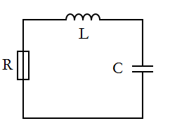
1[Figure 1]

The differential equation that governs this circuit is

LI''(t)+RI'(t)+\frac{1}{C}I(t)= 0 [1]

where L is the inductance, R is the resistance, C is the capacitance, I is the current through the circuit (which is the same at all places at one time since this is a series circuit), and t is the time.

Solving the Differential Equation

We can set arbitrary values for R, L, and C since they depend on the specific pieces of equipment themselves:

  • Inductance= 1 Henry
  • Resistance= 10 ohms
  • Capacitance= .1 farads

In Mathematica, the command to solve [1] looks like

\text{DSolve}\left[\frac{\text{Current}(t)}{\text{Capacitance}}+\text{Inductance} \text{Current}''(t)+\text{Resistance} \text{Current}'(t)=0,\text{Current}(t),t\right] [2]

which when solved, yields:

I(t)= c_1 e^{-8.87298 t}+c_2 e^{-1.12702 t} [3]

Completing the Full Solution via Graphical Solving

The two constants depend on the initial conditions of the circuit, which must satisfy Ohm’s Law of I=\frac{V}{R}. So, the initial current in the circuit must be 0.1 amps. Using a graphical guess-and-check method in Mathematica, I determined the value of the two constants to be approximately 0.05 each, resulting in a solution that is given by

I(t)= 0.05 e^{-8.87298 t}+0.05 e^{-1.12702 t} [4]

The plot of this equation gives us the current as a function of time, and looks like
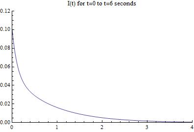
RLCCircuitsworking_finaldata1[Figure 2]

This graph tells us that although the RLC circuit starts out with a current of 0.1 amps, it quickly dies down due to the lack of a voltage source and is not very interesting after a few seconds. Refer to the upcoming conclusion blog post for a bit more analysis.

Now, lets examine the RLC circuit with a voltage source (much more interesting!)

RLC Circuit with AC voltage source

Circuit Diagram and Mathematics

Now we can model an RLC circuit that consists of a capacitor, voltage source, resistor, and an inductor. To easily visualize this, I have constructed a basic circuit diagram (Figure 3).
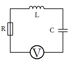
circuitwithnumbers1(Figure 3)

The differential equation that governs this RLC circuit is given by

LI''(t)+RI'(t)+\frac{1}{C}I(t)= E_{0} \omega cos(\omega t) [5]

where L is the inductance, R is the resistance, C is the capacitance, I is the current, \omega is the resonant angular frequency,  E_{0} is an initial value dependent on the voltage source, and t is the time. The inductance (L), resistance (R), and capacitance (C)are all determined by their respective circuit components, which are easily changed out for different ones. \omega depends on the inductance and capacitance, and its value is given by

\omega =\frac{1}{\sqrt{LC}} [6]

What we have left in terms of variables are current (I) and time (t). For our purposes, time is the independent variable, which leaves the current in the circuit at any time to be the dependent variable. Now that we have established this, we can solve our differential equation [5] for current as a function of time (I(t)).

Solving the Differential Equation

In order to solve [5], I will use the equation solving powers of Mathematica. In particular, the DSolve function is used.  When plugged into Mathematica, the input line looks like:

\text{DSolve}\left[\frac{\text{Current}(t)}{\text{Capacitance}}+\text{Inductance} \text{Current}''(t)+\text{Resistance} \text{Current}'(t)=E_{0} \omega \cos (\omega t),\text{Current}(t),t\right] [7]

We must set values for resistance, inductance, capacitance, and  E_{0}. For this solution, I chose the same values as the first circuit :

  • Inductance= 1 Henry
  • Resistance= 10 ohms
  • Capacitance= .1 farads
  •  E_{0}= 1 Volt

When the command is run with the above values set, Mathematica generates the general solution, which is:

I(t)=c_1 e^{-8.87298 t}+c_2 e^{-1.12702 t}+0.040824(-Cos(3.162t)+e^{6.661*10^-16t}Cos(3.162t)-0.3564Sin(3.162t)+2.806e^{6.661*10^-16t}Sin(3.162t)) [8]

First, lets make sure that this solution is reasonable. The known form of the solution to the equation for such a circuit is given by:

I(t)=c_1 e^{r_{1}t}+c_2 e^{r_{2}t}+Asin(\omega t-\varphi ) [9]

The form of our equation [8] seems to match up pretty nicely with this known solution [9]. Now, lets examine [8] in more detail.

Our solution [8] looks a little daunting, but we can break it down into its components. The first two terms have constants that depend on the initial current running through the system, i.e. when I(t)=I(0). However, we can approximate the equation by only looking at the last term, which is a superposition of sin and cosine functions along with a couple exponential terms thrown in. The reason that we can apply this approximation is that the first two terms “damp out” quickly, and thus have exponentially less of an effect as time progresses. The reader may still be curious to see how much of an effect these terms have on the current flowing through the system: to that I say don’t worry! After my initial approximation, I will solve for these constants and compare the two cases.

Approximate Solution and Graphs

For now, we will deal with the approximate solution, which is:

I(t)=0.040824(-Cos(3.162t)+e^{6.661*10^-16t}Cos(3.162t)-0.3564Sin(3.162t)+2.806e^{6.661*10^-16t}Sin(3.162t)) [10]

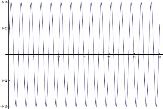
Now that we have this equation, we can use Mathematica to give us an idea of what the changing current looks like over a longer period of time. Figure 2 shows the current in the circuit as a function of time (I(t)) plotted over a 30-second interval.

30secondplot(Figure 4)

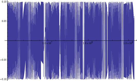
This looks like something we would expect! A sinusoidal wave that describes the changing current over time, just like our equations dictate. But, this is a short time-scale. What happens when we look at the changing current over a longer period of time? In Figure 3, I show the changing current over a longer time period (3000 seconds/50 minutes). In Figure 4, I repeat the process, but with the timescale being 5 years.
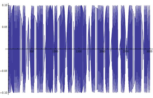
50minuteplot(Figure 5)

5yearplot(Figure 6)

In both Figures 5 and 6, we see some very interesting long-term variations in the current. Why does this occur?

Computational Limits

It is clear that Mathematica is displaying some odd variations that do not seem to have a set pattern. To investigate this and determine its cause, lets look closer at a range of time where the current seems to be irregular in the previous two figures. Specifically, lets look at the time scale between 300 and 400 seconds because it seems to have very strange behavior.
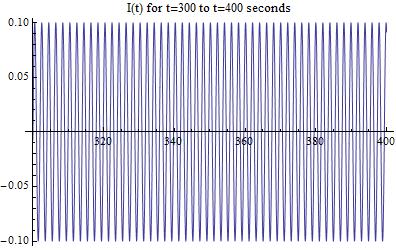
RLCCircuitsworking_finaldata1[Figure 7]

Looking at the graph above, we see that it looks completely normal! There are no strange variations and the current continues the predicted sinusoidal trend. This leads me to the conclusion that Mathematica has limitations that caused the irregular variations that we saw before, and that they do not actually exist in the data/circuit.

Completing the Full Solution via Graphical Solving

The next and final step in completing our model is accounting for the two initial terms that we left out. Lets take another look at the full equation.

I(t)=c_1 e^{-8.87298 t}+c_2 e^{-1.12702 t}+0.040824(-Cos(3.162t)+e^{6.661*10^-16t}Cos(3.162t)-0.3564Sin(3.162t)+2.806e^{6.661*10^-16t}Sin(3.162t)) [11]

We can see that they are exponential functions with a separate constant for each term. Solving for these constants quantitatively can prove to be difficult, so I will attempt to solve for them via a guess-and-check method using plots in Mathematica. I need to match the initial condition so that Ohm’s law is satisfied. So, I=\frac{V}{R} must hold in the initial state. This means that the initial current must be 0.1 amps. Lets try a few values for C[1] and C[2] and figure out graphically what they should be.

First, lets try values of 0.5 for each, resulting in the following equation:

I(t)=0.5e^{-8.87298 t}+0.5e^{-1.12702 t}+0.040824(-Cos(3.162t)+e^{6.661*10^-16t}Cos(3.162t)-0.3564Sin(3.162t)+2.806e^{6.661*10^-16t}Sin(3.162t)) [12]

The graph resulting from this equation is:
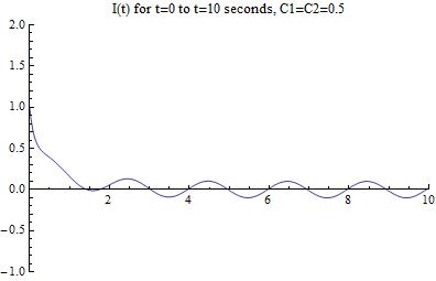
RLCCircuitsworking_finaldata6[Figure 8]

We can see that the initial current that this combination of constants is too high! It gives 1.0 amps, when we are looking for 0.1 amps.

Lets try slightly higher values for each, as well as having different values for the two. The equation that results is:

I(t)=2e^{-8.87298 t}+3e^{-1.12702 t}+0.040824(-Cos(3.162t)+e^{6.661*10^-16t}Cos(3.162t)-0.3564Sin(3.162t)+2.806e^{6.661*10^-16t}Sin(3.162t)) [13]

Which produces the following graph:
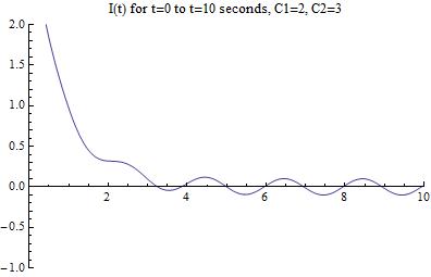
RLCCircuitsworking_finaldata7[Figure 9]

Looks like we have gone the wrong way with our guess! Lets try lowering both the constants to arrive at the correct graphical solution (in reality, this took me many more iterations of guessing and checking):

I(t)=0.05e^{-8.87298 t}+0.05e^{-1.12702 t}+0.040824(-Cos(3.162t)+e^{6.661*10^-16t}Cos(3.162t)-0.3564Sin(3.162t)+2.806e^{6.661*10^-16t}Sin(3.162t)) [14]

Which results in the following graph:
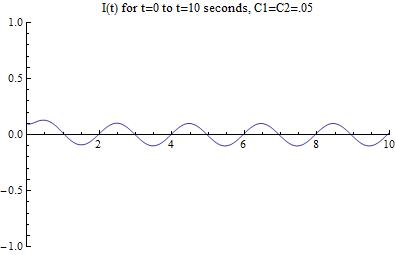
RLCCircuitsworking_finaldata8[Figure 10]

The Graphical Solution

Now that we have arrived at the correct graphical solution, lets change the scaling of the graph to better match that of [Figure 2], which was the initial approximation that did not take into account the two damping exponential terms.
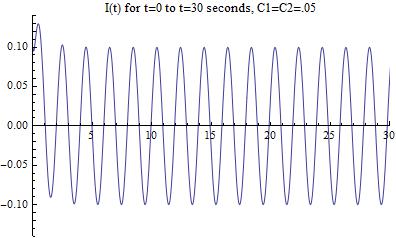
RLCCircuitsworking_finaldata9[Figure 11]


My conclusion from this final data will follow in my next blog post.


Resources

1. Circuit Diagram Maker- http://www.circuit-diagram.org/

2. The RLC Circuit- University of British Columbia-  http://www.math.ubc.ca/~feldman/m121/RLC.pdf

3. Mathematica Cookbook by Sal Mangano

4. Electronic Circuit Analysis for Scientists by James A. McCray and Thomas A. Cahill

5. Dynamical Systems with Applications using Mathematica by Stephen Lynch

6. Class Notes- Mathematics 228 (Methods of Applied Mathematics) taught by Matthew Miller


Mathematica Notebook

https://drive.google.com/file/d/0B3mtB6CQNnpjbXROcHl0VURzYlE/edit?usp=sharing

Share

Preliminary Results- RLC Circuits

Overview

In the following blog post, I discuss my progress with my project so far. I start out with a simple RLC circuit, go on to discuss the components, and derive a solution (using Mathematica) for a circuit with parameters that I have come up with. I then plot current as a function of time and discuss long-term structure in the output of the circuit, its relevance to my project, and my forward plan.

Progress

In my plan I discussed a simple RLC circuit that consists of a capacitor, voltage source, resistor, and an inductor. To easily visualize this, I have constructed a basic circuit diagram (Figure 1).

circuitwithnumbers1(Figure 1)

The differential equation that governs this RLC circuit is given by

LI''(t)+RI'(t)+\frac{1}{C}I(t)= E_{0} \omega cos(\omega t) [1]

where L is the inductance, R is the resistance, C is the capacitance, I is the current, \omega is the resonant angular frequency,  E_{0} is an initial value dependent on the voltage source, and t is the time. The inductance (L), resistance (R), and capacitance (C)are all determined by their respective circuit components, which are easily changed out for different ones. \omega depends on the inductance and capacitance, and its value is given by

\omega =\frac{1}{\sqrt{LC}} [2]

What we have left in terms of variables are current (I) and time (t). For our purposes, time is the independent variable, which leaves the current in the circuit at any time to be the dependent variable. Now that we have established this, we can solve our differential equation [1] for current as a function of time (I(t)).

In order to solve [1], I will use the equation solving powers of Mathematica. In particular, the DSolve function is used.  When plugged into Mathematica, the input line looks like:

\text{DSolve}\left[\frac{\text{Current}(t)}{\text{Capacitance}}+\text{Inductance} \text{Current}''(t)+\text{Resistance} \text{Current}'(t)=E_{0} \omega \cos (\omega t),\text{Current}(t),t\right] [3]

We must set values for resistance, inductance, capacitance, and  E_{0}. For this run through of the solution I chose the following arbitrary values:

  • Inductance= 1 Henry
  • Resistance= 10 ohms
  • Capacitance= .1 farads
  •  E_{0}= 1 Volt

When the command is run with the above values set, Mathematica generates the general solution, which is:

I(t)=c_1 e^{-8.87298 t}+c_2 e^{-1.12702 t}+0.040824(-Cos(3.162t)+e^{6.661*10^-16t}Cos(3.162t)-0.3564Sin(3.162t)+2.806e^{6.661*10^-16t}Sin(3.162t)) [4]

First, lets make sure that this solution is reasonable. The known form of the solution to the equation for such a circuit is given by:

I(t)=c_1 e^{r_{1}t}+c_2 e^{r_{2}t}+Asin(\omega t-\varphi ) [5]

The form of our equation [4] seems to match up pretty nicely with this known solution [5]. Now, lets examine [4] in more detail.

Our solution [4] looks a little daunting, but we can break it down into its components. The first two terms have constants that depend on the initial current running through the system, i.e. when I(t)=I(0). However, we can approximate the equation by only looking at the last term, which is a superposition of sin and cosine functions along with a couple exponential terms thrown in. The reason that we can apply this approximation is that the first two terms “damp out” quickly, and thus have exponentially less of an effect as time progresses. The reader may still be curious to see how much of an effect these terms have on the current flowing through the system: to that I say don’t worry! After my initial approximation, I will solve for these constants and compare the two cases.

For now, we will deal with the approximate solution, which is:

I(t)=0.040824(-Cos(3.162t)+e^{6.661*10^-16t}Cos(3.162t)-0.3564Sin(3.162t)+2.806e^{6.661*10^-16t}Sin(3.162t)) [6]

Now that we have this equation, we can use Mathematica to give us an idea of what the changing current looks like over a longer period of time. Figure 2 shows the current in the circuit as a function of time (I(t)) plotted over a 30-second interval.

30secondplot(Figure 2)

This looks like something we would expect! A sinusoidal wave that describes the changing current over time, just like our equations dictate. But, this is a short time-scale. What happens when we look at the changing current over a longer period of time? In Figure 3, I show the changing current over a longer time period (3000 seconds/50 minutes). In Figure 4, I repeat the process, but with the timescale being 5 years.

50minuteplot(Figure 3)

5yearplot(Figure 4)

In both Figures 3 and 4, we see some very interesting long-term variations in the current. Why does this occur? Well to be honest, I am not completely certain. I do have a few ideas though:

  • My first inclination is that the long-term variations are in part due to the approximation I made by removing the first two terms of Equation [4].
  • My second idea is that these long-term structures are present due to a possible approximation Mathematica may have made when solving the differential equation.
  • My third and last thought is that these variations are not an artifact of finding the solution, but truly do exist in this theoretical circuit I have chosen.

Why?

A question that the reader may have after looking at all of this is “Why is the long-term structure important?” The answer lies in the fact that RLC circuits are embedded in many electronic devices, including radios and televisions. For this reason, it is important to know the current they put out. We don’t  really want something that has an unpredictable output in devices that are high-cost.

Forward Plan

To further investigate the reason for the long-term structure, I will first solve for the constants in Equation [4] and plot the graphs of current again. Hopefully this will provide some insight into the workings of the circuit. I may also alter the initial parameters (inductance, resistance, etc.) to see if this provides any insight. If not, then I will investigate Mathematica’s differential equation solving techniques and attempt to alter my solution in a way that provides a more accurate solution.

Resources

1. Circuit Diagram Maker- http://www.circuit-diagram.org/

2. The RLC Circuit- University of British Columbia-  http://www.math.ubc.ca/~feldman/m121/RLC.pdf

3. Mathematica Cookbook by Sal Mangano

Mathematica Notebook

https://drive.google.com/file/d/0B3mtB6CQNnpjejEzN25zbFlqajQ/edit?usp=sharing

Share

Project Plan: RLC Circuits

Plan/Goals:

In this project, I plan to study the relevant differential equations that govern RLC circuits and use Mathematica to solve them for values that are useful. The general equation governing a basic RLC circuit with a capacitor, voltage, resistor, and inductor in series, in that order is:

LI'(t)+RI(t)+\frac{1}{C}Q(t)=V(t) [Equation 1] (UBC- Source 4)

which, when going through a series of substitutions, becomes:

LI''(t)+RI'(t)+\frac{1}{C}I(t)=\omega E_{0}cos(\omega t) [Equation 2] (UBC- Source 4)

Equation 1 has six variables: L (inductance), R (resistance), C (capacitance), V (voltage), Q (charge), and I (current). When a circuit like this is set up in the lab, the values that are known are L, R, C, and V because they directly depend on the components of the circuit. Once the differential equation [2] is solved, values for current (I) and charge (Q) can be determined. I will use Mathematica to solve for the general solution to this differential equation [2], which is a second-order differential equation. Once I have the general solution, I will vary the initial conditions to determine the effect of different circuit components on the overall properties of the circuit. Following this, I will develop more series RLC circuits with components that are set up differently in terms of their component structure.

Timeline (Weeks 1-5):

Week 1: I will begin by reviewing basic differential equation solving techniques for first and second order differential equations. I will also study the differential equation solving capabilities of Mathematica and review the techniques for solving second-order differential equations as they apply to RLC circuits.

Week 2: I plan on solving for the general solution to Equation 2 above (using Mathematica). I will vary different initial conditions and create graphs that visualize the changes that occur. I will also have a visual representation of the circuit.

Week 3: Develop another series circuit or study a previously built one. Determine the general equation for it and begin the solution process.

Week 4: Finalize the solution for the second circuit. Develop graphs for visualization purposes.

Week 5: I will finalize my project by proofreading all the components and making sure everything is presentable. I will also provide constructive criticism to my peers on their projects.

Sources:

1. Mathematica Cookbook by Sal Mangano

2. Electronic Circuit Analysis for Scientists by James A. McCray and Thomas A. Cahill

3. Dynamical Systems with Applications using Mathematica by Stephen Lynch

4. The RLC Circuit- University of British Columbia- http://www.math.ubc.ca/~feldman/m121/RLC.pdf

5. Class Notes- Mathematics 228 (Methods of Applied Mathematics) taught by Matthew Miller

Collaborators:

N/A


Share

Developing Models of RLC Circuits

For my project, I will study RLC circuits. RLC circuits have three main components; resistors, inductors, and capacitors. These circuits are important because of their prevalence in radios and televison (among other things). Specifically, I will develop a few different configurations of these circuits and measure characteristics such as voltage, current, resonance, and most importantly, damping. The physics that governs RLC circuits relies heavily on the mathematics of differential equations. For this reason, Mathematica, due to its strong capabilities in regards to differential equations, is the ideal program to use to model and study these systems.

Share