Optical Filters

Now that we have the theory down, let’s apply convolution to actual data. The model here is two optical filters placed on top of each other. The light beam will go through both filters, and come out the other side somewhat convoluted. I have chosen two optical filters from thorlabs:

• Item #FGB37-A: BG40 Colored Glass Filter, AR-Coated: 350 – 700 nm
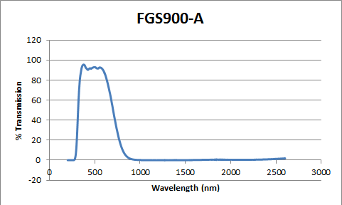
• Item#FGS900-A: KG3 Colored Glass Filter, AR-Coated: 350 – 700 nm

The plots of their transmission percentage as a function of wavelength are shown below:

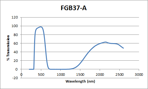
Notice the first plot down does not tend to zero as the wavelength increases. My hypothetical light beam will have a wavelength of around 500 nm, so I cropped out the two peaks from each plot from 200 nm to 1000 nm. I also added 200 zeroes to each end extending my plots from 0 to 1200 nm. I did this so that the transformations would have as little noise as possible.

Convoluting the two functions requires using the exact same method described earlier, but instead using discrete Fourier transformation. My first attempt at convoluting these two plots failed. The convolution gave me complex solutions, and I need my solutions to be real. I tested the method on two Gaussian functions by extracting artificial data points through the function ‘Table’. The list of data presented was not in the same format as the imported optical filter data. Mathematica does not like Excel, and the data imported was in the format of a list of 1×1 matrices of each point [The data also needed to be one dimensional, so the x-axis represents data point number. Fortunately the amount of data points is equivalent to the range of wavelengths, so for all intents and purposes the x-axis represents wavelength]. To bypass this confusion I saved my data as a text file and imported the list as a list. For example:

a = Import[“C:\\Users\\Zeeve\\Desktop\\EM Project\\FGB37-A test.txt”, “List”]

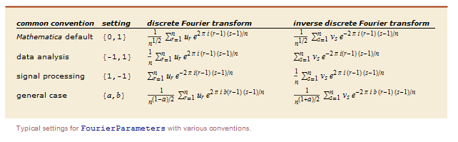
The data is now real. It should also be noted that the default setting for the Fourier transform is not the convention for data analysis. This requires using the tool FourierParameter to change the range from {0,1} to {-1,1}.

 

This is what my data looks like:

 

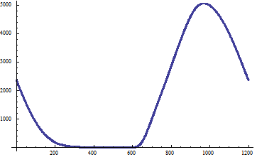
The y-axis is the transmission percentage, and the x-axis is the wavelength.

Notice the peak is around 1000 nm. It turns out that the inverse discrete Fourier transform of the product of two Fourier transforms of data is not the convolution of the data. It is actually the cyclic convolution of the two data sets. If you go back to the original definition, one of the functions in the integral of the convolution is shifted by some value x’.

Notice also the y-axis and how it extends to beyond 5000. This is because my normalization constant was wrong. The square root of 2 Pi in the convolution algorithm is a normalization constant for Gaussian functions. Correcting this was simple. I used the ‘Normalize’ function to normalize my Fourier transforms, and used the product of those results:

v = Normalize[m]*Normalize[n] instead of c=Sqrt[2 Pi] m*n

Correcting the former issue is trickier. I need to cycle the function back to peak at around the 500 mark. I admit I am not familiar with the mathematically correct method of correcting this error, so I ball-parked it. The peak needs to be around 500 nm since the original data peaked at around 500 nm. Cycling the curve backwards required outside help. I used the method described in the first answer here: http://mathematica.stackexchange.com/questions/33574/whats-the-correct-way-to-shift-zero-frequency-to-the-center-of-a-fourier-transf .

The method uses the function ‘RotateRight’ to cycle a range of data a certain amount of points. My range of points extends from 0 to 1200, and I cycled 400 points. Now I have a plot where the x-axis is pretty much the correct wavelength for its corresponding value (although the values are off by a factor of 100, which is fine since it is simply a normalization correction), which is the convolution of the two optical filters:

 

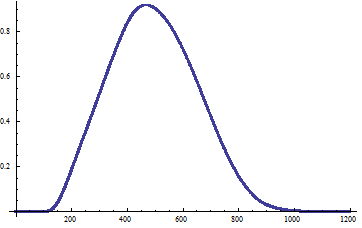
Again here the y-axis is the transmission percentage, and the x-axis is the wavelength. The y-axis is off by a scaling factor.

For a complete transcript of the convolution, please check out the Mathematica script:

https://vspace.vassar.edu/zerogoszinski/Optical%20Filters.nb

Here are the text files:

https://vspace.vassar.edu/zerogoszinski/FGS900-A%20test.txt

https://vspace.vassar.edu/zerogoszinski/FGB37-A%20test.txt

Future:

For my conclusion I will discuss about deconvolution and some expansions on convolution.

Note: If the files do not work for you, I have uploaded all of my files to Google Drive which can be accessed in the conclusion. The concerning files are the Mathematica script ‘Optical Filters’, and the two text files ‘FGS900-A test’ and ‘FGB37-A test’.