Gauss’s Law is a powerful tool for understanding electric fields for all types of configurations. The most general case of Gauss’s Law is given by $ \oint \! \textbf{E} \cdot \mathrm{d} \textbf{a} = \frac{1}{\epsilon_0} Q_{enc} $. In this equation, $ \textbf{E} $ represents the electric field vector, $ \mathrm{d} \textbf{a} $ represents the differential area vector of the Gaussian surface through which the electric field is pointed, $ \epsilon_0 $ represents the permittivity of free space, and $Q_{enc}$ represents the charge enclosed by a Gaussian surface.
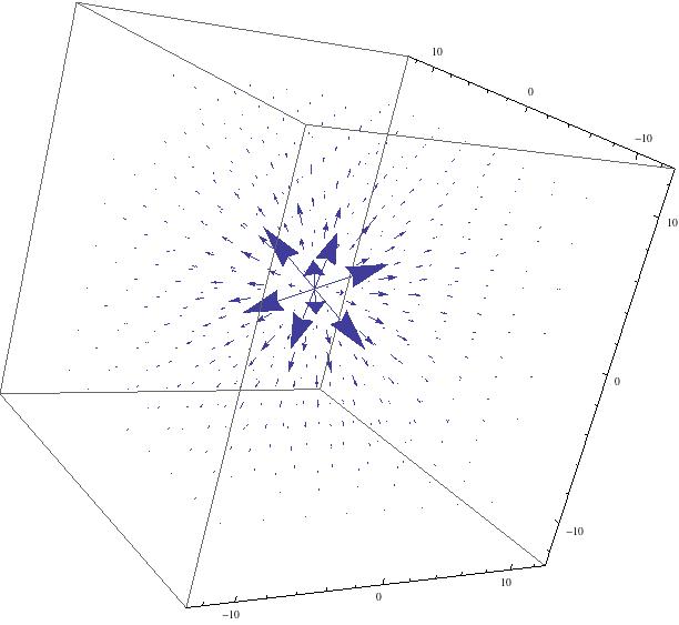
As stated in my project plan, the general case can be used to solve for the electric field of a point charge, which is given by $\textbf{E} = \frac{1}{4 \pi \epsilon_0} \frac{q}{r^2} \mathbf{\hat{r}} $. The unit vector indicates that the electric field for a point charge points in the radial direction. In my project, I managed to use this equation to model the electric fields for both positive and negative point charges.
I also worked to model the electric field for hollow spherical conductors. The above equation still holds, but with one caveat:

In the above, $R$ represents the radius of the sphere. This piecewise function describes the fact represented in Gauss’s Law that a electric fields only exist in regions in which a charge is enclosed. In conductors, all of the charge exists at the outer surface, so there is no electric field on the inside of a hollow spherical conductor. When the distance away from the conductor is greater than its radius, it obeys the second piece of the piecewise function.
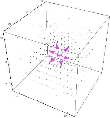
This image shows the electric field produced by a positive point charge in free space.
My project was initially intended to be a project that produced visualizations of the above equations. From that point, I intended to develop more complex systems, work out the math for them, and then visually model them as well. However, due to my inexperience with Mathematica 9, I encountered many issues. The RegionFunction proved to be my saving grace, as described in my results post, but it happened too late for me to be able to model more complex systems.
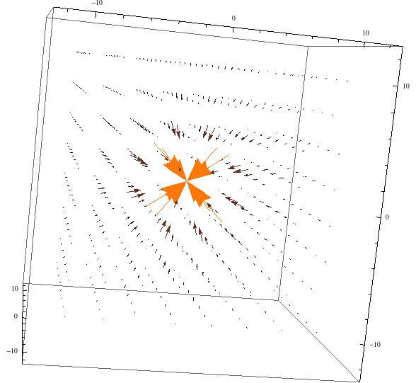
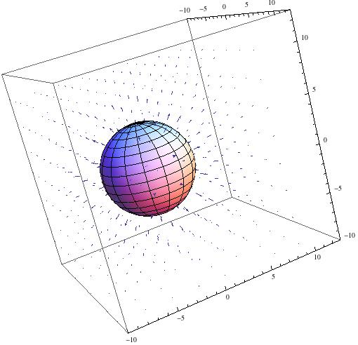
This image shows the electric field produced by a negative point charge in free space. Compare to the figure for a positive point charge.
My results do show good visual models for electric fields of single positive and negative point charges, and a positively charged spherical conductor. These visual models are incredibly useful tools for understand electric fields. Looking at an equation (Gauss’s Law) can only do so much for one’s understanding; a visual strongly aids this.
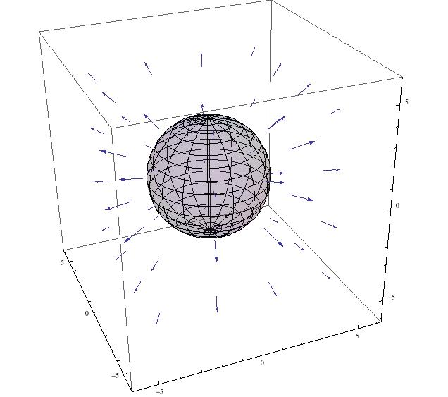
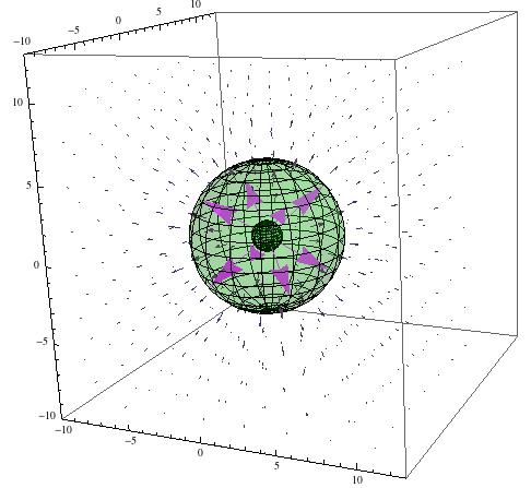
This shows the electric field produced in free space by a spherical conductor with positive charge on the surface.
I wish that Mathematica had even more tools for visually modeling these electric fields. I tried to create an animation that showed the graphing of the vector field arrows coming out of the point charge, but this did not work. I don’t believe Mathematica’s VectorFunction3D works with its Animate function, but it may just require different inputs. I also tried to create a Manipulate object to demonstrate changes in the electric field as charge changed, but this was also not successful. Part of me believe this is an issue of scaling the image, and part of my believes that this function is also not compatible with VectorFunction3D.
In the future, this project could be expanded by modeling more complex systems. One way to complicate this would be to introduced additional spherical conducting shells with charge on them. Another complicating factor would be to put a point charge inside of a spherical shell. These systems could be modeled with differing signs and values of charges. Additionally, an infinite charged plane could be added to show other ways the electric field might change.
Additional investigations could also include modeling the electric fields of dielectrics instead of conductors. This analysis would be especially complex because it would include polarizations and bound charges. Additionally, this could include the modeling of the electric displacement in addition to the electric field.
Sources and Resources:
- Introduction to Electrodynamics, David Griffiths, 4th Edition
- Mathematica 9: Student Edition, created by Wolfram
- Collaborators: Brian Deer and Tewa Kpulun