
By using the formula for the magnetic field of a wire that I derived in my preliminary data,
(1) 
I was able to model systems composed of current-carrying wires.
First I used the above equation and converted from Cylindrical to Cartesian coordinates. This was done because Mathematica will only plot vector fields in this form. I then plotted the resulting vector field due to a positive current.
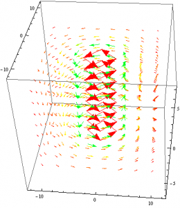
This is exactly what we would expect to see for the magnetic field of current carrying wire as illustrated by the well known “Right-Hand-Rule”. The field lines are more intense towards the center of the of the wire while they decrease exponentially as they move further away. They are also oriented counter-clockwise since a positive current was used. Suppose now that we were to switch the current to a negative value.
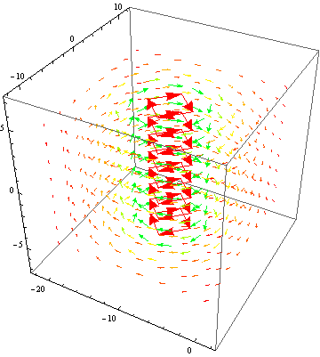
As expected, the field lines behave in the same way as before expect they oriented in a clockwise fashion.
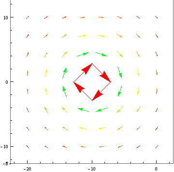
Below I changed the viewpoint of the magnetic field such that only the x,y plane is shown. This helps to visualize the field because the field does not change along the z-axis.

Now that I successfully found the Magnetic Field for a current-carrying-wire, I could make the system more complicated by adding additional wires.
Suppose that some identical wires were placed parallel to each other at some distance.
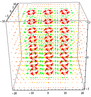
Again I changed the viewpoint such that only the x,y plane is seen. 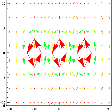
As you can see in the above plots, the fields in between the wires have a certain type of symmetry. The field lines point in opposite directions and as they get closer to the midpoint between the to wires, they are of the same magnitude and cancel. It is safe to assume that as the distance between the wires approaches 0, the magnetic field between the wires will no longer exist.
Above and below the set of wires, the direction of the field lines due to each wire is the same: +x below the wire and -x above the wire. Coincidentally, this shares similar traits to the magnetic field due to a plane of current; the field lines above and below the plane will point either in the positive or negative x direction while there is no magnetic field anywhere along the plane itself. This shows that a plane of current can be viewed as a collection of parallel wires with no distance between them.
Suppose now that I had two wires parallel to each other but rather than having both wires having the same current, they are opposite to each other.
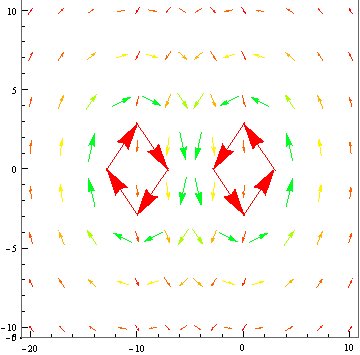
If Mathematica were able to superimpose the magnetic fields from the different wires, I suspect that the resulting field would resemble that of a magnetic dipole. However, I have not been able to find a function that will do this given two different vector fields and am limited by time to model a magnetic dipole using an alternative method. Nevertheless, the field that I was able to model does share some similarities to that of a dipole. The symmetry of the field lines are the same as those of a dipole. This is a result of two equal and opposite currents.
References:
- Griffiths’ Introduction to Electrodynamics 4th edition
