
The next step of my project involved applying the modeling and manipulation code to different scenarios. In this case, I chose two scenarios that started as purely electric and developed magnetic components when considered in moving reference frames. The first was a continuous case- an infinite parallel-plate capacitor, and the second was a discrete case- a single point charge.
As has been well established, the field between two capacitor plates of charge density +/-σ is E=σ/2ε0. It is unsurprising then, that the E-field of a capacitor looks like this:

It is equally unsurprising that since there is no moving charge, there is no B-field. Then, when the system is considered in a reference frame moving at speed v relative to the capacitor and the transformation equations are applied, the following fields emerge for E…
and B…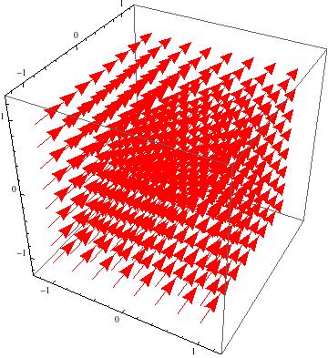
These look pretty dull, but are a few things to note about these figures. The first is that Mathematica is not able to show absolute magnitude of the vector fields: just the relative magnitude. That is, the arrows are the correct size relative to the other arrows in the box, but they are not necessarily to scale when compared to other fields. This is why the plots appear unchanged when v changes: the values of the vectors are all changing, but all at the same rate, so the pictures do not change.
The second notable feature is that (without accounting for the actual magnitudes of the fields), it is possible to see that even though the E- and B-fields both change, the direction of the net force does not. For a positive test charge at rest in the reference frame moving in the x-direction, it would experience only an electrostatic force in the z-direction in the rest case. For the moving case though, it would experience an E-field still in the z-direction and a B-field in the y-direction, both of which would result in a net force that is still in the z-direction.
Despite the simplicity of a point charge, this third case is actually the most interesting to look at because it is not infinite, but discrete. Thanks to every intro E&M course we’ve ever taken, we know that the E-field created by a test charge is E=q/r24πε0. The following vector plot or something similar probably appears in every intro textbook currently on the market.
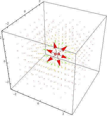
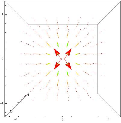
Pretty boring, right? Completely spherically symmetric and falls off with r2 as expected. Now for the interesting ones: the fields in a moving reference frame. The E-field actually starts losing gaining so much of a y- and z-component that it appears to flatten out in the x-direction. The following figure is for v=0.75c
The B-field does something equally strange: it becomes somewhat cylindrical. However, in my code, this only appears at very high v (greater than 0.96c).
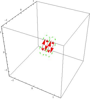
I get the feeling that if I could make mathematica show more detail, the field would not be in a perfect cylinder though. Since two rings of vectors appear on either side of the origin, it may be that the actual field has two lobes of some sort that are symmetric about the x-axis.
The last thing to note about this model is that when v=c, the simulation returns an error because it has to divide by zero when calculating gamma. Furthermore, the expression for gamma returns imaginary numbers for v>c, so this model is not useful for considering hypothetically how a system might behave if anything were able to move faster than the speed of light.
The mathematica worksheet associated with this can be found here.

Mathematica certainly has its limitations; however, you can find additional (better ways) to visualize the relativistic effects to bring your point across. You can click on the right hand brackets to delete the part of your code that you want to delete. See Ms. Johnson for help.