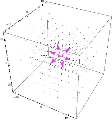
I began by modeling the electric field for a point charge +q, equal to the value of an elementary charge.

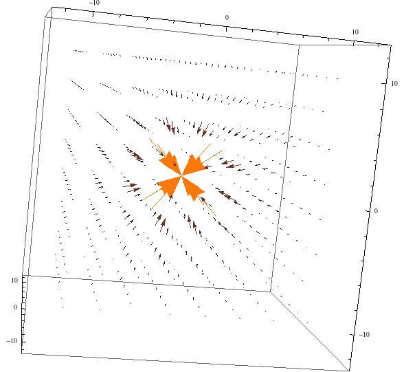
I also modeled the electric field of a point charge of -q.

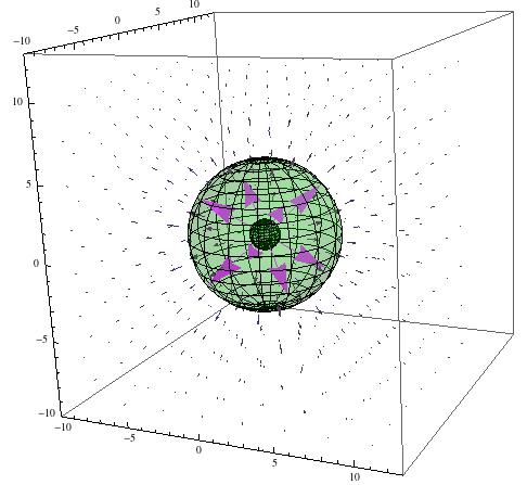
Next, I attempted to model the electric field due to spherical hollow conductor with total charge +q. First, I graphed a sphere of radius 5 using Mathematica’s SphericalPlot3D function. I superimposed the electric field of a positive point charge over this sphere, knowing that this would be incorrect. By Gauss’s Law, the stated configuration would result in an electric field of 0 inside of the spherical conductor, and an electric field following $\textbf{E} = \frac{1}{4 \pi \epsilon_0} \frac{q}{r^2} \mathbf{\hat{r}} $ for r > 5. The following image shows a partially transparent sphere with an electric field inside of it, violating Gauss’s Law.

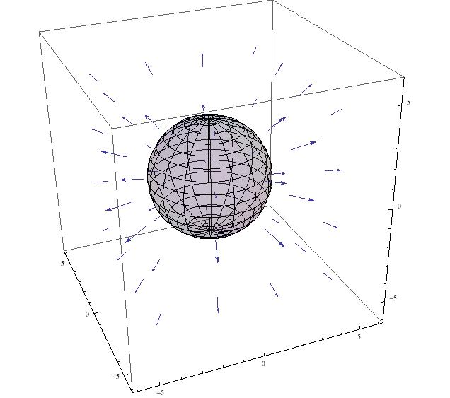
However, thanks to Brian Deer, I learned to use Mathematica’s RegionFunction, which allowed me to specify which regions of the graph on which the vector function would apply. The following now shows a hollow conductor of radius 3, with an electric field only present outside of it. Unfortunately, this step took a lot of time to work out, as I tried many different ideas to only get the field to show for certain radius values (i.e. be 0 inside of the conductor). I was unaware of RegionFunction, and even when I did learn what it was, I had trouble getting it to work with my model.

My updated Mathematica file can be found here.