Final Models(Updated) | Modeling and Experimental Tools with Prof. Magnes

Magnetic Field for a Cylindrical Conductor:

LONG CYLINDER:

Using Ampere’s Law I derived the magnetic field for a simple system, a long cylinder with the current uniformly distributed on its surface. Using Eq. 2, I was able to solve for the magnetic field. The results are as follows:

A) For s < r, B=0

B) For s > r, $B=\frac{\mu _{0}I}{2\pi s}\hat{\phi }$ (1)

$\oint B\cdot dl=\mu _{0}I_{enc}$ (2)

In Figure 1 , we have a ContourPlot of the magnetic field of a long cylinder with a current I distributed on the surface of the cylinder. Assuming that the current is flowing into the screen we know that the magnetic field is in the positive ϕ direction. If the current were coming out towards us, the magnetic field would be in the negative phi direction.

Figure 1. This is a 2D contour plot that shows the flow of the B-field outside of the long cylinder. Look at this as if you were looking down on the cylinder with the current flowing into the screen.

Figure 2. Is another way of demonstrating what is happening to the long cylinder. This picture depicts the gradual decrease of the magnetic field’s magnitude as we move away further . The arrow curving around the top of the cylinder represents the direction of the B-field when the current is going into the screen.

Methods:

Using mathematica I was able to demonstrate these physical occurrences. Before developing the above figures I tried showing the magnetic field using the StreamPlot function, however that resulted in an oval like shape for the positive ϕ direction. The arrows are pointing in the right direction but the pattern formed does not represent the magnetic field for our situation. As you can see in Figure 3, the center of the plot starts of as a circle but as the radius of the cylinder increased the stream looses it’s circular shape and starts to flow like an ellipse.

Figure 3. This is a StreamPlot of the B-Field outside of the long cylinder. This is not a correct illustration of what is happening to the wire because it’s shaped like an ellipse.

Before entering my results into mathematica I changed from cylindrical coordinates to Cartesian coordinates using the TransformedField function. With this, my results are now

$B=\frac{\mu _{0}I}{2\pi \sqrt{x^{2}+y^{2}}} \widehat{\phi }$

Similar methods were used for the electric field.

Electric Field for a long cylinder:

Using Guass’ Law I derived the electric field inside of a long wire with charge density $\rho =ks$ , for some constant k. Using Equation 2, I got the equation $E_{inside}=\frac{ks^{2}}{3\epsilon _{0}} \widehat{s}$ .

$\oint E\cdot da=\frac{1}{\epsilon _{0}}Q_{enc}$ (2)

With this I modeled Figure 4, where the vectors point radially outwards of the cylinder. Figure 4, illustrates what happens in the center of the wire.

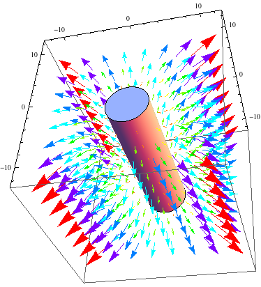
Figure 4. This is the Gaussian cylinder within an actual cylinder, where the magnitude of the E-field increases as the Gaussian cylinder approaches the size of the actual cylinder. Think of the axes as the parameters for the actual cylinder.

FINITE CYLINDER:

ELECTRIC FIELD FOR A FINITE CYLINDER:

After looking at the models for the long wire and talking to Professor Magnes about my blog I did modeling for an actual cylinder with parameters. For the E-field, the Cylinder is 30cm in length with a radius of 10cm. It has a charge density of $\rho =ks$ , which is the same as the long wire, only now confined to certain limits. After doing the math to find the E-field outside of the cylinder ( s > r ), I got

$\mathbf{E}=\frac{kl_{1}r^{3}}{sl_{2}\epsilon _{0}} \widehat{s}$ ,

where the k is a constant (where k = 1), $l_{1}$ is the length of the cylinder ( $l_{1}$ = 30cm), $l_{2}$ is the length of the Gaussian cylinder ( $l_{2}$ = 40cm), r is the radius of the Cylinder , and s is the radius of the Gaussian cylinder.

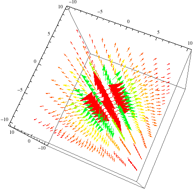
Figure 5. This is the E-field of a finite cylinder. As you can see here the magnitude of the E-field decreases the further you move away from the cylinder.

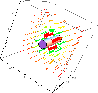
Figure 6. I placed the cylinder within the plain from Figure 5 to show the E-Field moving radially outward. I altered the size of the cylinder to have a better view of what’s going on.

MAGNETIC FIELD FOR A FINITE CYLINDER:

Here’s the magnetic field for a finite cylinder, with the same parameters as the one for the E-field. This is a cylinder with a current distributed uniformly across the surface of the cylinder. For this cylinder, I made the current (I) equal to 1A. After using Ampere’s law I got the same results as that of equation 1 from above.

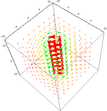
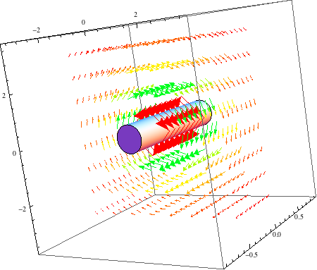
Figure 7. The image on the left demonstrates the B-field of a cylinder. The image on the right shows the field on the left acting on a cylinder with set limits.

In this mathematica file you will also find a ContourPlot3D of what’s happening with the B-field. This file also contains the work I did for a Finite Cylinder.

To view the work I did in mathematica click on this link for the Electric Field:https://drive.google.com/file/d/0B2VxS7Y5dxIHMTZxUEFyb21yZWM/edit?usp=sharing

To view the work I did in mathematica click on this link for the Magnetic Field: https://drive.google.com/file/d/0B2VxS7Y5dxIHU0wxOTRHY0ZxdjA/edit?usp=sharing

1 thought on “Final Models(Updated)”

Jenny Magnes May 5, 2014 at 12:36 pm

Include a description with every figure. It does not seem like your animated plot represents an accurate description of how the field is changing. You can easily export your animations as a gif or movie file. I don’t see the animations anymore. I am confused about what you are actually modeling here. Is this a finite cylinder or an infinitely long wire? What is the magnetization?

Comments are closed.