The previous presentation of results was very limited–limited in the scope of the actual results that were presented, and limited in the scope of analysis. Here, I present further results with a greater analysis of implications, limitations, etc.

First, let us consider why we care about such a scenario. A sphere is a relatively simple object, but also a very interesting one. Many other objects can be modeled as spheres, or as a combination of several. For me personally, I have been working with a spherical microphone, and since I wish to understand how the sound behaves on the surface of this microphone, I need to take into account how the sound is scattering from the microphone. This is the main practical application I am familiar with, though there are bound to be others.

An acoustic plane wave is very simple and is best shown with an image rather than an equation. Note it is very much like it sounds (no pun intended): a plane (in the mathematical sense) traversing through the air.

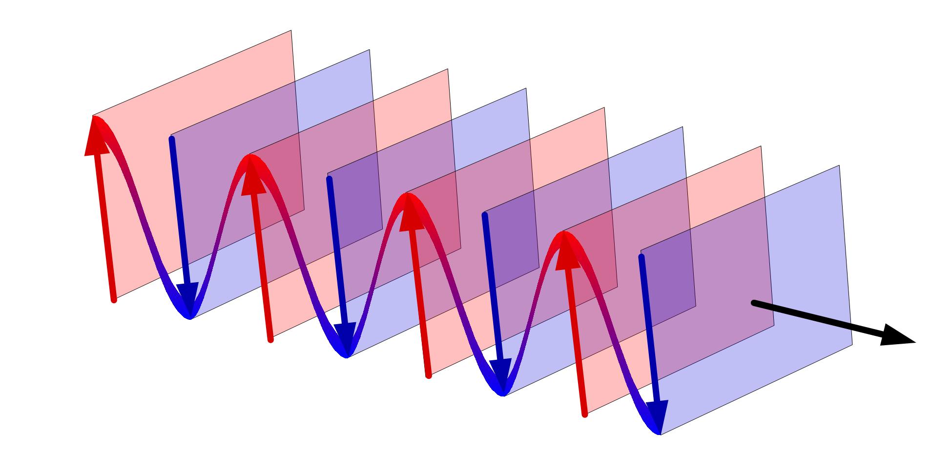
Source: commons.wikimedia.org

Now, to understand how this plane wave interacts with a sphere, we need several things: 1) for convenience and simplicity, a way of describing the plane wave using spherical coordinates; 2) a series of functions known as spherical harmonics; 3) and to meet a couple of boundary conditions called the Dirichlet Boundary Condition and the Sommerfeld Radiation Condition.

I won’t go into detail here about 1) and 3), but shall simply show results below. As for spherical harmonics, they are to 3 dimensions what Fourier Series are to 2 dimensions: they allow us to break apart 3D shapes or fields into an infinite series of functions. For more on spherical harmonics, see the end of this post.

The equation describing the pressure field at the surface of a rigid sphere (after being struck by plane wave) is as follows:

Where i is the complex unit, n is a term representing the sum index as well as the spherical harmonic order within the sum, k is the wave-number of the acoustic plane wave, a is the radius of the rigid sphere, m is the degree of the spherical harmonic, Θ_k is simply the (theta, phi) pair representing the direction of incoming sound, Θ_s are the (theta, phi) pairs of every point at which we’ve chosen to evaluate the pressure field (or the “sampling points”), and Ynm is the spherical harmonic of order n and degree m. Finally, bn(ka) is given by:

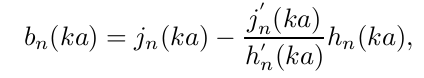
where jn and hn are the type one spherical Bessel and Hankel functions, respectively, and the apostrophe (‘) denotes their derivatives. Note that this pressure field is the very solution we want–that is, the equation of very near field scattering and diffraction all in one. In fact, it is actually a superposition of incident energy and reflected energy (for more on this, see reference [1] below.

Now, in principle this first equation is exact; it yields perfect solutions with no errors. In practice, however, we must approximate this solution on several levels:

1. We must truncate the sum in the first equation, as finite computing power only allows finite calculation of spherical harmonics and bn,
2. The Spherical harmonics, spherical Bessel and Hankel functions (jn and hn) must be approximated, as they do not have a simple analytical form,
3. The number of points at which we can evaluate the pressure field on the surface of the sphere must be finite (e.g. would could choose 64 evenly spaces points, or 128, etc.); ideally we could choose infinite points

Our main priority here are bullet points 1. and 3. Matlab does a very good job of approximating the Spherical Bessel and Hankel functions, and the error attributable to them is small in comparison with the other two errors. Let’s discuss points 1. and 3. in detail (they shall be discussed together since they are related):

Let N be the maximum spherical harmonic order, or the maximum order of our sum (replacing the infinity in equation 1).

For small N, there are huge errors in the calculated sound field because the spherical harmonics fail to truly estimate the shape of the sound field. They simply can’t produce the detail fine enough. Let’s illustrate the point graphically. Below are the cross-sectional graphs for N=0, 1, 2, and 10 for the sound pressure field at the surface of the sphere, for a plane wave of frequency 1000 Hz.

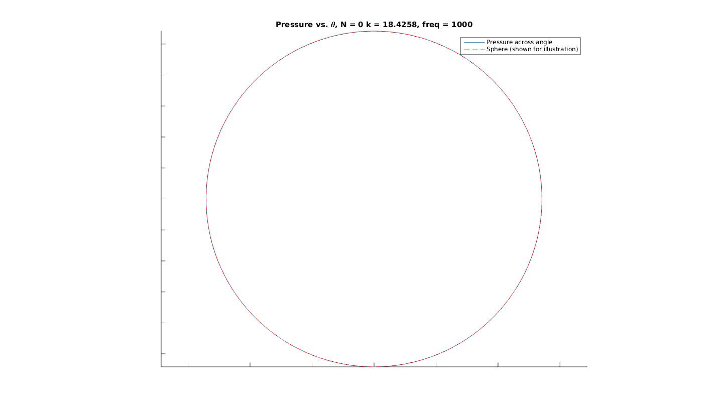
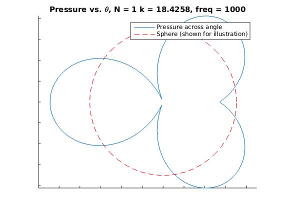
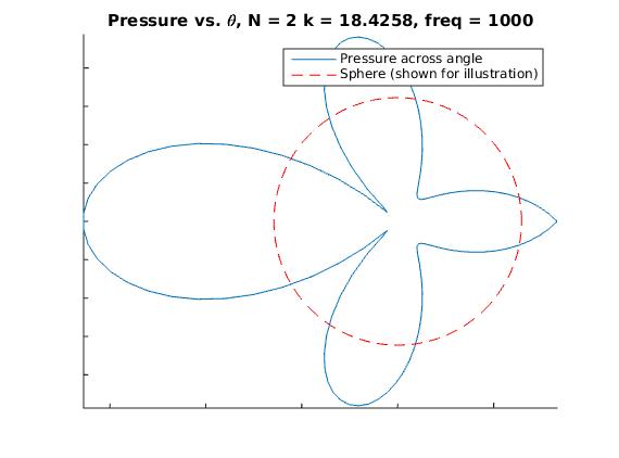
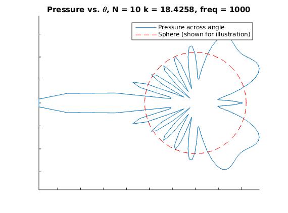
Notice how the first few graphs fail entirely to capture the true detail of the sound field, whereas the final graph is quite detailed. Spatial errors of this sort, due to the truncation of the sum of spherical harmonics, are called spatial Aliasing Errors.

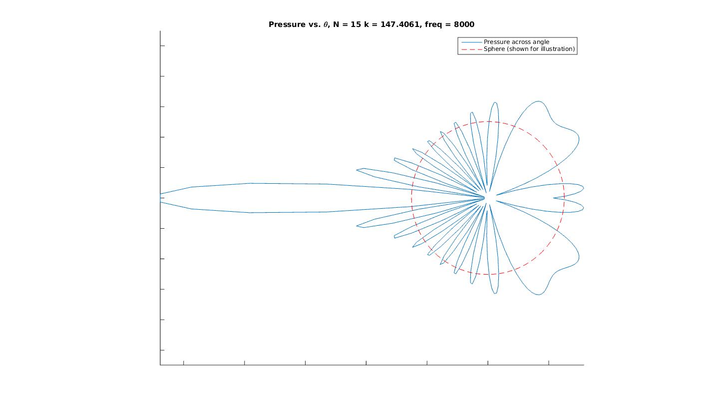
Another type of spatial aliasing occurs when we try to examine high frequency sound. Since we only have a finite number of points to work with, higher frequency sound tends (or shorter wavelength) to be harder to model. The reason is this: as the wavelength gets shorter, it begins to approach the distance between our samples (if we’ve chosen 64 evenly spaced points, for example, there is finite distance between each point). Once this happens, we no longer have enough samples to reconstruct the sound field. This behaviour is akin to the Nyquist Frequency and sampling rate: signals with a frequency higher than the Nyquist Frequency simply can’t be reconstructed accurately. Let’s look at this graphically as well. Below are the cross-sectional graphs for N=10, 20, 30, and 100 for the sound pressure field at the surface of the sphere, for a plane wave of frequency 20000 Hz. 128 Sample points have been used.

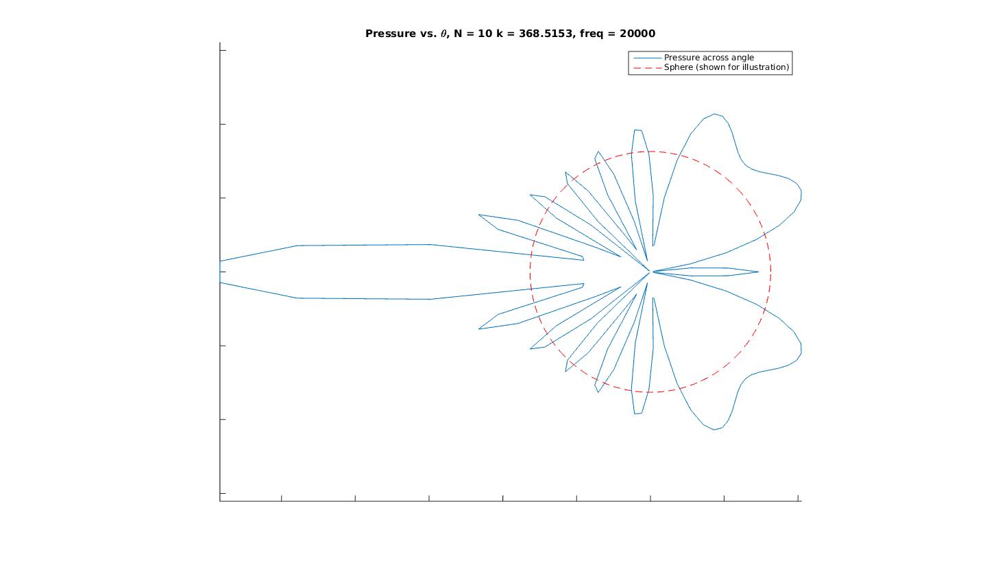
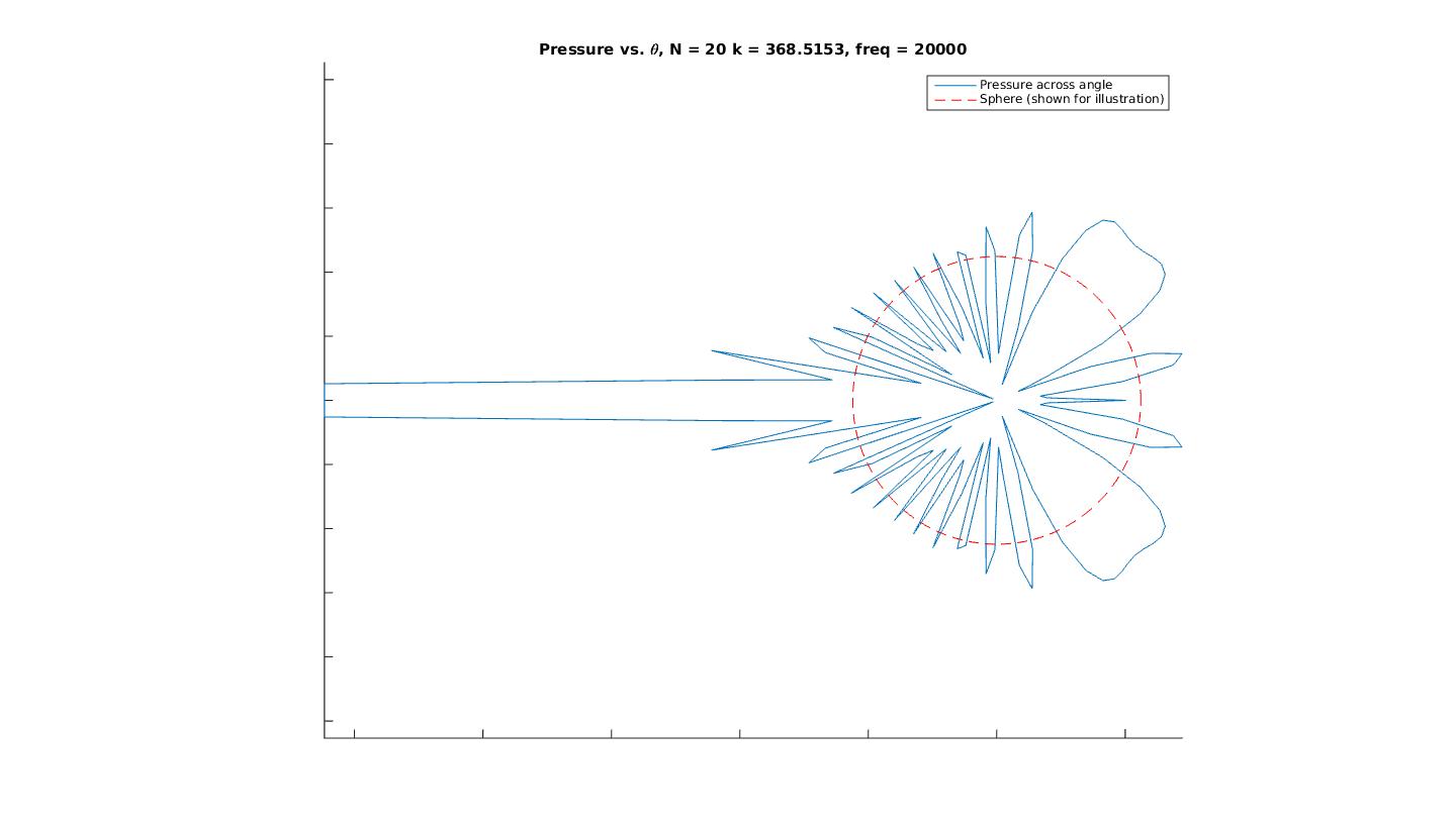
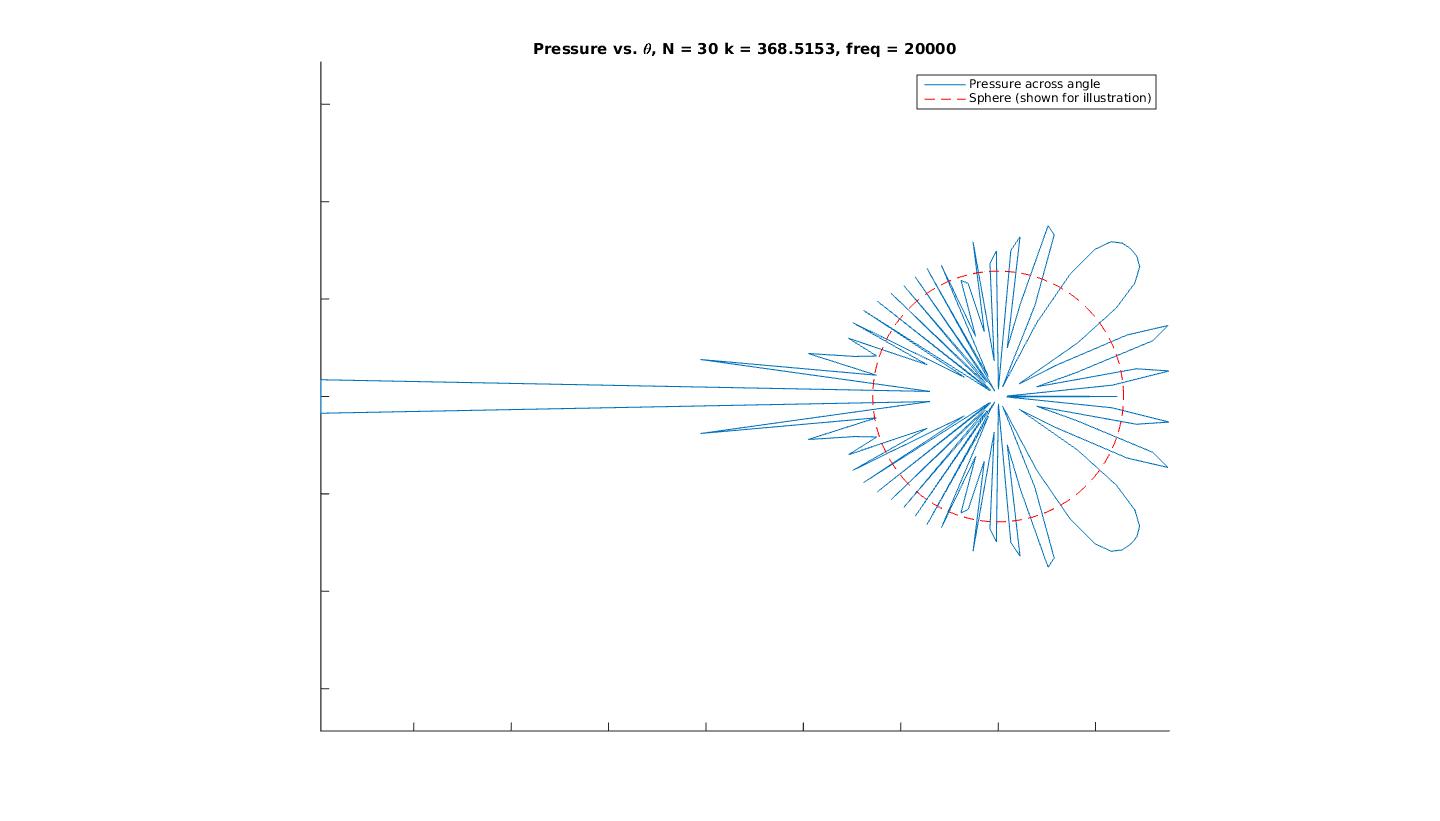
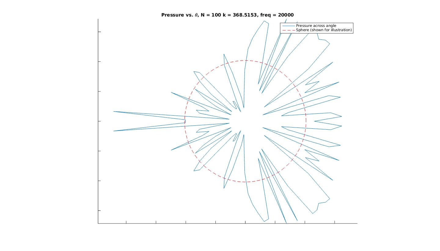
It’s looking good, it’s looking good… and it fails. We’ve maxed out our capability to model the sound at 20000 Hz, and further addition of spherical harmonics, after a certain point, actually gives us worse results.

So, it was seen in practice that choosing a maximum order of approximately N = sqrt(M)-1, where M is the number of sampling points, was ideal for most cases. Addition of higher orders may lead to frequency related spatial aliasing as shown above, though in practice it has been observed that somewhat higher values of N may (a few orders more) may also be acceptable [3].

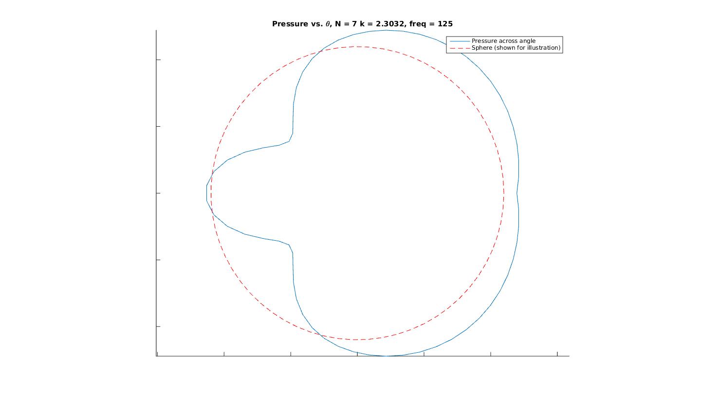
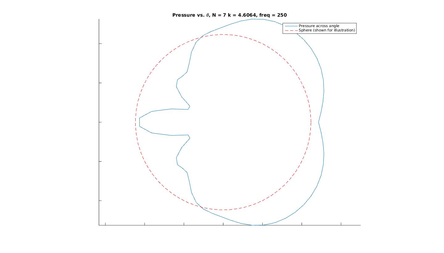
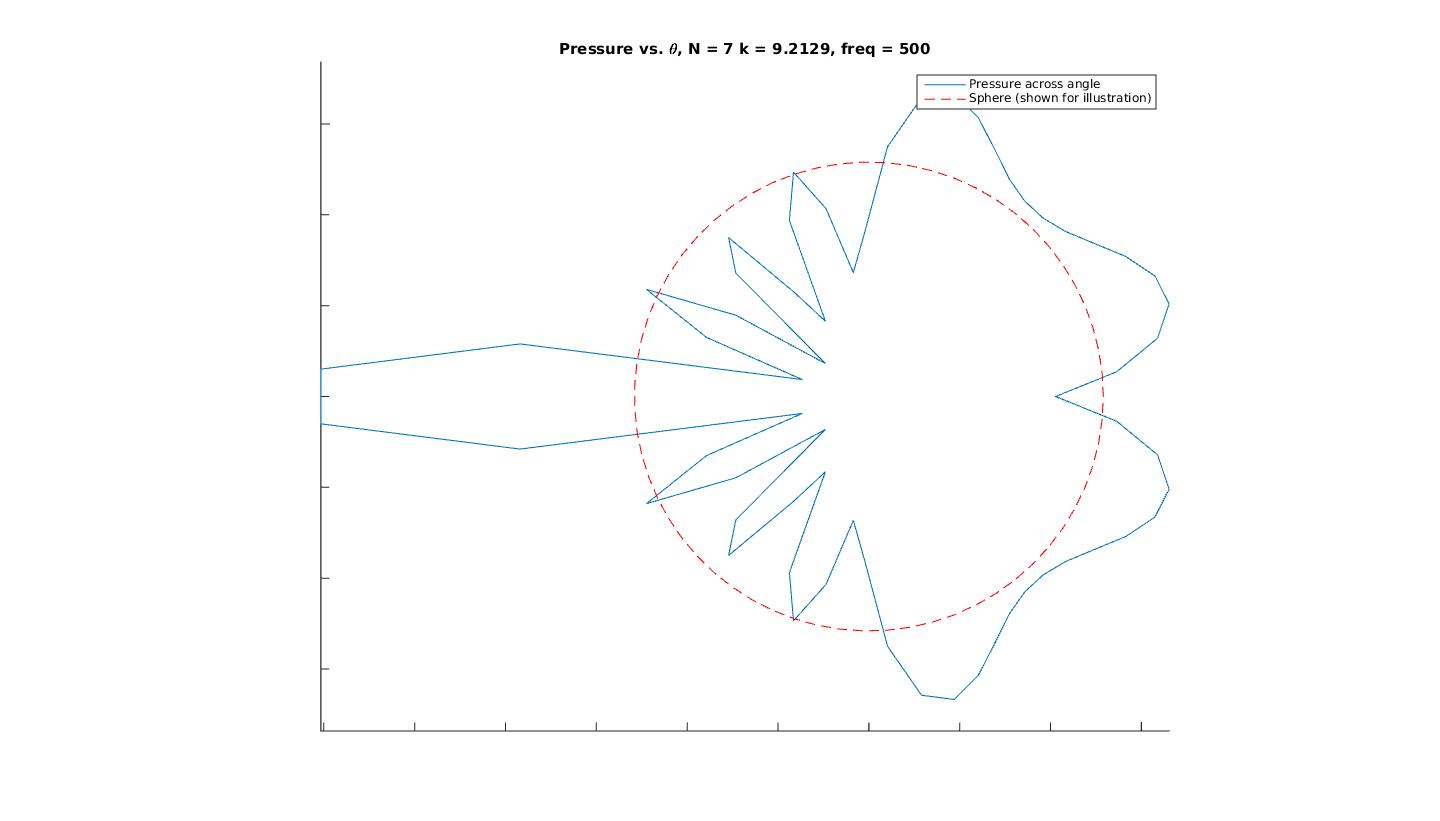
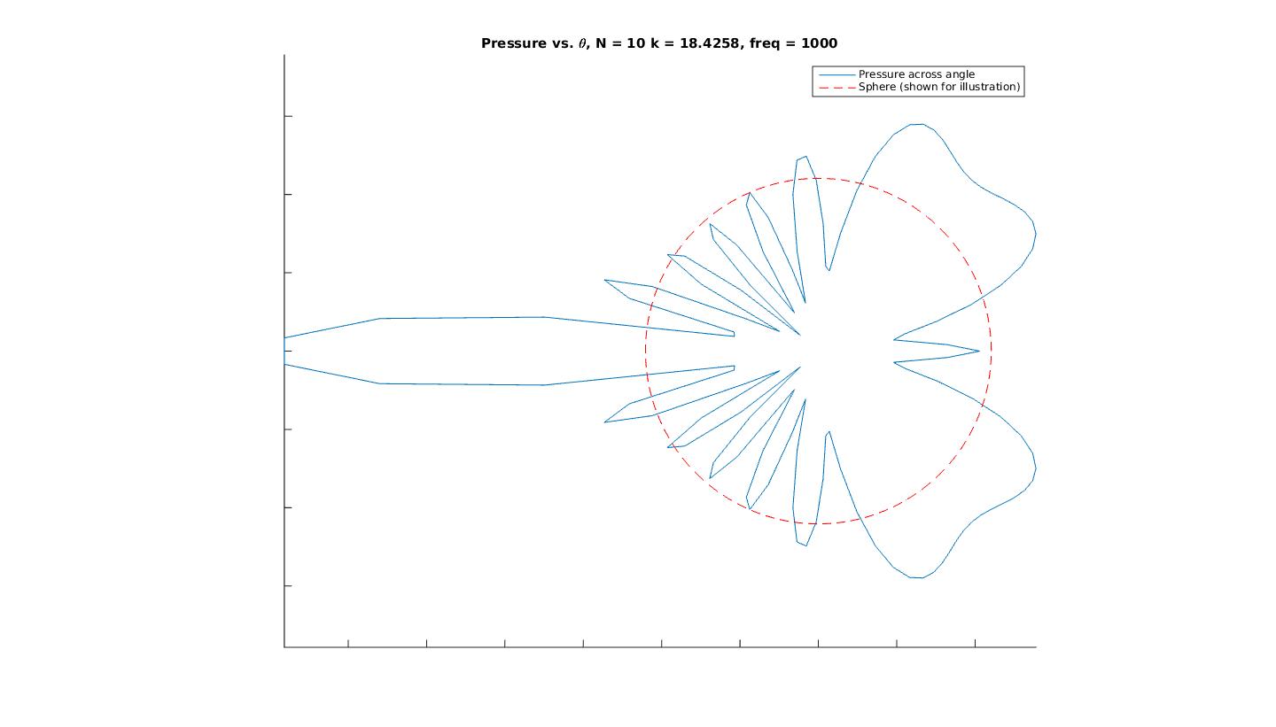
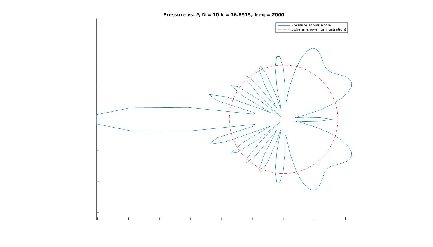
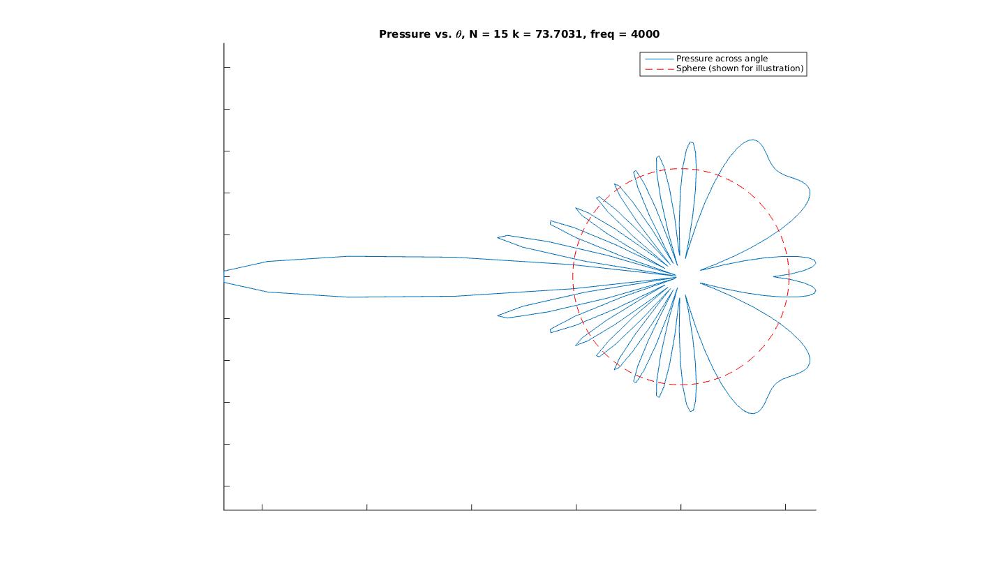
Below are graphs for the 2D cross sectional area of the sound pressure at the sphere, and the corresponding sound field around the sphere. Results are shown for octave bands between 100 and 8000 Hz (125, 250, 500,1000, 2000, 4000, 8000), the frequency range most important for human hearing. Number of sampling points and N have been adjusted periodically to improve resolution.

Sound field on sphere:

Contour plot of sound field in vicinity of sphere (x and y axes are simply xy-coordinates in meters):

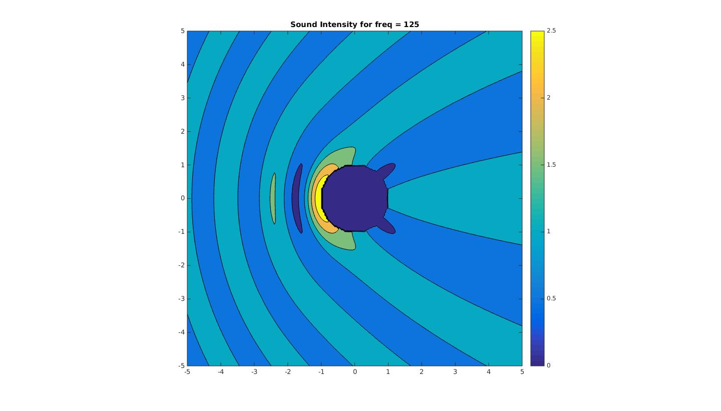
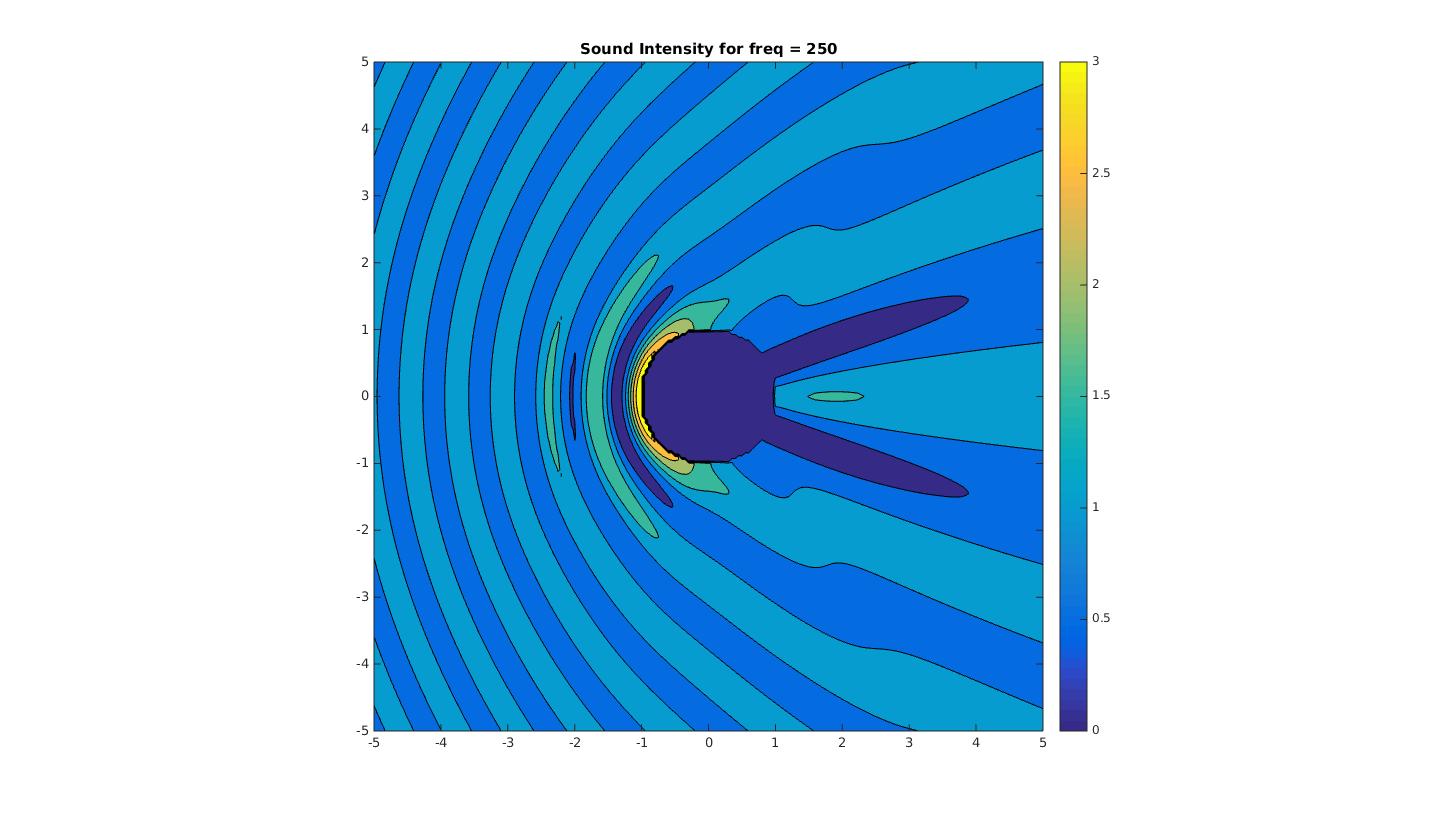
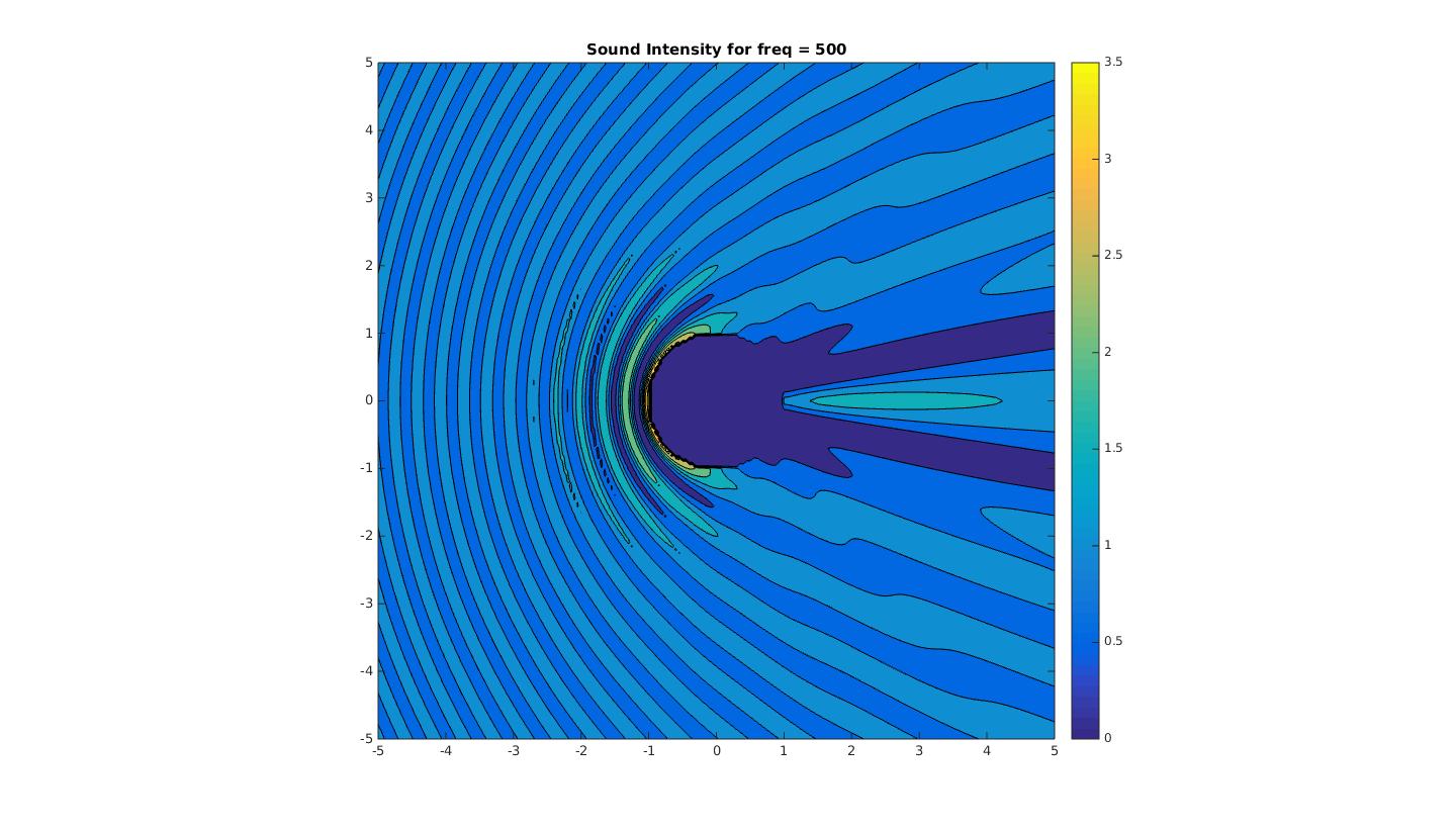
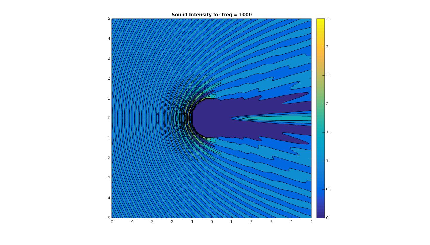
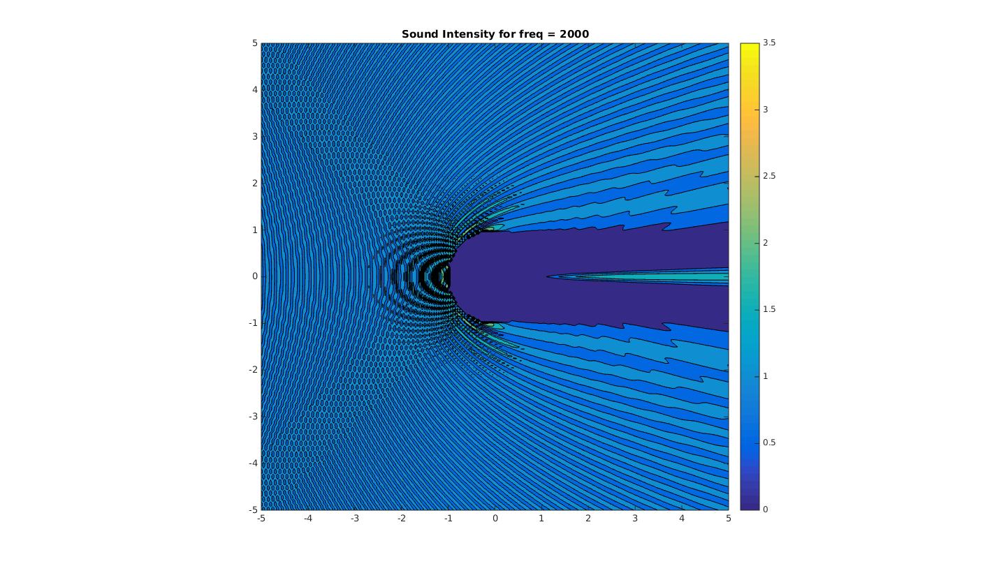
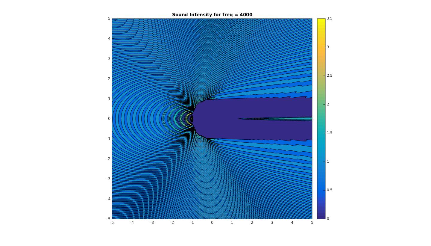
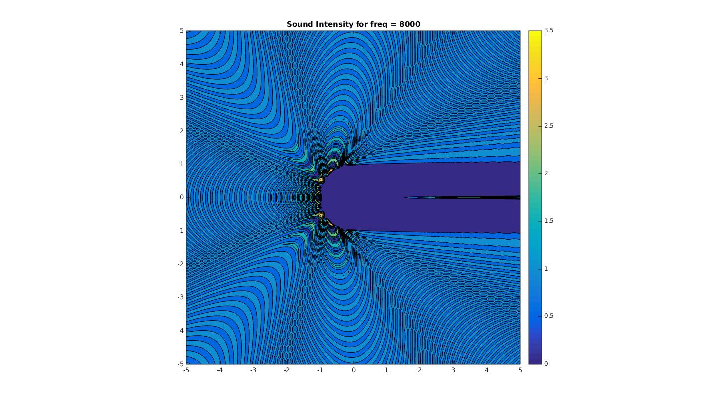
Notice how, for low frequency (long wavelength) the scattering is actually quite low. This should make a lot of sense physically, since the larger the wavelength with respect to the sphere, the more likely the sound is to simply diffract around the sphere and “ignore” it altogether. On the other hand, for higher frequency (shorter wavelength), the scattering becomes quite large, especially at the front of the sphere. This should also make sense, because the spherical boundary becomes more and more like a flat surface to a smaller and smaller wavelength, and hence reflects sound approximately back in the incident direction. Note too that for high frequency there much less diffraction than for low frequency.

TODO: more in depth analysis of error, especially numerically. Clean up code. Comparison to limiting case of Rayleigh scattering.

—————————————————————————————

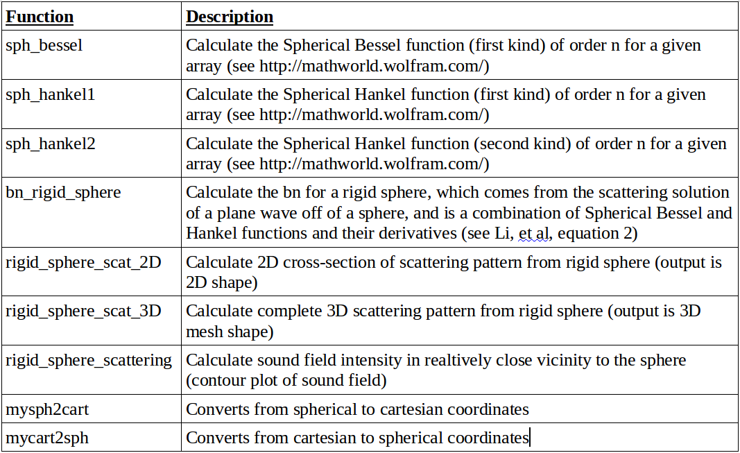
NOTE: Here is a table describing the function of the code. Below the table is a link to the updated code, which have vastly improved commenting to facilitate use. I would recommend using rigid_sphere_scat_2D over its 3D counterpart, simply because the 2D is so much easier to visualize, and since the scattering is symmetric, it tells essentially the same info.

Link to code:

https://drive.google.com/a/vassar.edu/folderview?id=0B3UNwnkM9fLrfkRlb05LdEVOTzhCQWRuRHRCVVFjUDJIMHBpWlF2V3ZKd3UwWXNwVWRua28&usp=sharing

Spherical Harmonics [2]:

Note that spherical harmonic order starts at 0, not 1.

References:

[1] http://ansol.us/Products/Coustyx/Validation/MultiDomain/Scattering/PlaneWave/HardSphere/Downloads/dataset_description.pdf

[2] http://mathworld.wolfram.com/SphericalHarmonic.html

[3] O’Donovan et al. Imaging concert hall acoustics using visual and audio cameras.

[4] Li et al. “Fast time-domain spherical microphone array beamforming.” IEEE Workshop on Applications of Signal Processing to Audio and Acoustics. 2007

Alex Molina & Kadeem Nibbs
Computational 375 – Project

GOAL: Week 2: Run simple trial with one-dimensional object in two-dimensional space with air resistance ( varying wind speeds and air densities)

In all track events run/jumped primarily in one direction, wind is an important consideration in athletic performance. In the long jump, and in the shorter sprinting events (the 60m, 100m, 200m, and all of the similarly distanced hurdle races), the maximum allowable tailwind (wind propelling the athlete forward), is +2.0m/s. There is no maximum allowable headwind (wind pushing the athlete back), but at headwinds stronger than -5.0m/s, an event might be postponed. For our latest results presentation, we compared the jump trajectories while varying wind assistance and air density, in each case holding all other variables constant.

Our original goal for the week was to improve our model to have a 3D projectile with limb objects, functions to bend and extend the limbs, and methods to calculate the cross-sectional area and center of the mass of the body depending on the state of the limbs. However, we could not figure out how to implement object-oriented design in MatLab, and we failed to properly define functions in our code, which made our prospects shaky at best. We instead decided to learn what information we could from our current working model.

Our results showed that wind assistance has a major impact on performance in the long jump, as a jump into a 5m/s headwind netted a distance of about 5 meters, a mediocre distance for a male high school jumper, and a jump propelled by a 2m/s tail wind recorded a distance of nearly 25 feet, which is an elite college-level distance. We found that air density had a negligible effect on the jump distance, variations of up to 50% in air density resulted in less than a millimeter difference. This reaffirms what we learned in introductory mechanics, that air resistance is negligible in most cases of projecting motion, the exceptions being when the air is moving, and when the object is moving at high speeds. Air resistance will not significantly affect an athlete jumping at 20mph into still air. This also shows that although air density can be as high as 1.2kg/m^-3 at cities near sea level, and as low at .75kg/m^-3 at cities 5000m above sea level, long jumps performed at any city in the world can be compared because of air density’s negligible effects on performance.

Important Links:
MatLAB code and other essential information can be found at:
https://drive.google.com/open?id=0B6loGd4o7iESfjNoRnVmSjJDNHlabG9qNEJIRmY1Z1JEeS1QNE9rTjlIY2Vqc1NMTWlwdEk&authuser=0

References:
Giordano, Nicholas J., and Hisao Nakanishi. “Chapter 2: Realistic Projectile Motion.” Computational Physics. 2nd ed. Upper Saddle River, NJ: Pearson/Prentice Hall, 2006. Print.

Our Resulting Projectile Motion with Varying Wind Speed:

Our Resulting Projectile Motion with Varying Air Density:

UPCOMING: Week 3: 
Run a second trial with a mass-less two dimensional object in 3-dimensional space. We will more to run two test trials with three-dimensional object in three-dimensional space, each with different body position.

Unfortunately, I was unable to finish hacking the equipment in the laboratory to harvest EMG signals. This is because I do not have access to LabView hardware in my lab yet, and as such am currently unable to read my own surface EMG signals onto a computer. However, the sample signals mentioned previously in the preliminary data proved sufficient to proof this code and derive an understanding of the capabilities of this version of the algorithm. Pictured below is the absolute value of a sample EMG spectra (EMGSample1.mat), which allows a viewer a better understanding of the kinds of trends within the signal easier.

I was successfully able to create a working code that finds the peak amplitudes above a contraction threshold, and the thousands of separate cycle durations distinguished in order for each of the the three states of action in the robotic arm, contracting, holding at a contraction, or resting/ returning to resting. Like the previous iteration of code, this version implements a FFT (Fast Fourier Transform) noise analysis process to help eliminate the primary sources of noise in the EMG signal, 60 electronic noise and low frequency (<20 Hz) vibrations. Although significant, the effects of this noise cancellation is not sufficient to fully extinguish all experimental noise. For this data, I cannot include any further analysis as I do not know the lab conditions from which this data originated. Pictured below a snippet of the raw EMG spectra is shown above that same data after being passed through a rectification process. Although noise is still an issue in the rectified signal, the rectified data is more workable than its predecessor. However, since a Fourier transform is a frequency analysis tool, I have had to abandon running a truly continuous analysis in favor of chopping the data up into smaller bins of some small time and going through the analysis process for each bin individually as a quasi continuous process.

For the purposes of testing the efficacy of the EMG analysis code, the noise threshold, which determined whether the arm would be in the resting state or holding some strained state, was made lower than it ought to be in a practical experiment. Similarly, the threshold that determines when the signal indicates contraction was lowered, such that there would be more opportunities within each signal to evaluate if the code was executing as intended. The data for both peak amplitude and cycle duration is saved in a 20 by j matrix, where j is the number of bins that characterizes the stagnant code in this iteration, or in a later version the number of bins that have been created up to this point.  For cycle duration, the data is stored for each bin as a column vector in a matrix, with elapsed time for contraction cycles, rest cycles, and holding cycles stored in order (values 0-1 contraction, 1-2 holding, 2-3 resting). Similarly, the values for peak amplitude during the contraction cycles are stored with the same indices as the contraction duration that they occur during. The peak amplitudes are represented as a proportion of the contraction threshold, which will allow for easier programming of the robotic arm downstream.

The data sets are inordinately large, so I will leave it to the discretion of the reader to use Google drive to access the code and run the results. However, the image below is a screenshot of the results for cycle durations of the first data set (SampleEMG1.mat) between 1.85 and 2 seconds. Although this code serves its purpose, it is not a perfected or completely stable arrangement. Due to the large datasets and indexing method used, changing noise threshold outside of a small range around .1 can or altering the algorithm that controls the analysis can cause the code to crash.

Furthermore, as a byproduct of ensuring a higher degree of stability such that the code is reasonably likely to function properly over a dataseries, the cycles are trimmed slightly and lose resolution in each bin. To compensate for this, any excess time in each bin that has not been accounted for is said to be a hold state at the end of the bin. Though this may seem inefficient, This extra time at the end of each bin will allow the physical system and computational analysis to stay at pace with one another, as the extra hold time can be reduced while the physical system tries to continue a motion. Further work on this code will include making it more robust and resilient, as well as finishing on getting my own EMG signals to analyze. Outside of the context of this class, I plan on integrating the analysis code with the code to control the robotic arm, as well as increasing the sophistication of my model such that the outputs and conclusions better correlate with physical action in a biological agent.

Relevant Files can be found through the link below with headers:

1: EMG_Data_Analysis_422.m

2: SampleEMG1.mat

3: SampleEMG2.mat

4: SampleEMG3.mat

https://drive.google.com/drive/#folders/0B0K4JjJfDy1ffkR4eEZaMzlxb0xvTjRjWDBIUm9iVzZuRmVyeG1aM0RhWHMxcVB6RXZDUFk

References:

1: De Luca, C. Gilmore, D. Kuznetsov, M. Roy, S. Filtering the surface EMG signal: Movement artifact and Baseline noise contamination. Journal of Biomechanics (January 5, 2010) 1573-1579

2: Richards, C. Biewener, A. Modulation of in vivo power output during swimming in the African clawed frog. Journal of Experimental Biology 210 (2007) 3147-3159

3: Lichtwark, G. Wilson, A. A modified Hill muscle model that predicts muscle power output and efficiency during sinusoidal length changes. Journal of Experimental Biology 208 (2005) 2831-2843

4: Computational Physics by Nicholas J. Giordano and Hisao Nakanishi

Nadav Hendel & Matteo Bjornson

Week Two

The celestial two body problem can be solved exactly, allowing us to observe Kepler’s Laws in action, but the same is not always true of the three-body case. Thus, solving the three body problem exactly has been a central problem of celestial mechanics. In this section, we model the effect of adding a third planet into our system. We will use Jupiter, since it has the largest mass of the planets and therefore would have the most significant effect on the Earth and Sun. The planetary motion will still be related using the inverse square law for gravitational force, and the sun will still be fixed to the origin for our first routine Jupiter-Earth.

Jupiter-Earth is very similar to our first routine Planets, in terms of methodology. For each time step, the planets positions are calculated using the Euler-Cromer method. This is completed by keeping track of the distances between both planets and the sun, as well as the interplanetary distance. From these distances, we can compute the acceleration of each planet as related by the inverse square law, and from there, the new positions. The code for this program is quite dense, and as noted in the textbook, it can be more efficient to define some recurring variables at the beginning of the code such that they need not be recalculated during each iterative loop. Despite this we opted not to do this in our code for the sake of clarity since this added efficiency is quite small.

From our initial results running this program, we can see that using normal masses for Earth and Jupiter, stable planetary orbits can be achieved. At this point, we will continue our experimentation by observing how a change in Jupiter’s mass would affect the Earth’s orbit. As an initial point of reference, a small increase of ten fold of Jupiter’s mass yields negligible results, as Jupiter’s mass is still dwarfed by that of the sun.

In the textbook, a mass increase of 1000 fold is supposed to yield much larger changes in the earths orbit. Unfortunately, we were not able to achieve this result exactly, and were only able to note significant changes using a mass of closer to times 9000 Jupiter original mass. The results of this are shown below:

The fact that we had to increase the mass of Jupiter to 9000 to observe noticeable changes in earth’s orbit indicates that we may  still have some bugs in our code that need correcting. According to Giordano, these effects should have been visible at 1/10th that mass.

Now that we have established this model, we also wished to explore what a true-three body system would look like with our second routine. As the mass of Jupiter approaches that of the Sun, or at the very least significant in comparison, it is unreasonable to simulate this system with the Sun fixed at the origin. The difference between the 3-Body Orbit  routine and the Jupiter-Earth routine is that the center of mass is now set as the origin, and we also incorporate the movement of the sun as it is affected by the enlarged mass of Jupiter. The Sun is given an initial velocity so the net initial momentum is zero, keeping the center of mass from leaving the origin. A few interesting things can happen to this system when the initial conditions are adjusted.

The first change we attempted to make with the model was to establish a base case, simply by multiplying the mass of Jupiter by 100. An increase of mass of this magnitude was intended to perturb earth and the sun, but not by much. As you can see below, this change actually had significant effects on both the sun and Earth’s motion. Despite this, the Earth’s motion with respect to the sun still appears very regular.

One of the first things we noticed was extreme sensitivity to initial conditions. In the following two gifs, the mass of Jupiter is multiplied first by 710x, and second by 710.2x. As you can see, this difference of .2 yields a largely different path for the Earth. In fact, it seems that the results from this section are much closer to the chaotic regime than expected due to their sensitivity. This observation might have some insight into why these systems are so hard to calculate in general.

In exploring the effects of different initial conditions, we set the initial velocity of the Sun to zero. We observed the Sun to follow a cusped path, which seemed almost unnatural. Is this even possible? This also made us realize we need to establish a deeper understanding of the implications of giving the Sun an initial velocity.

These investigations have revealed another discussion we were not expecting to find: how do we know these simulations are correct? Or, how do we know the effects we are observing are not artifacts of the numerical approximation or specific lines of code introducing error? Looking forward to next week we need to investigate ways we can can validate our code and results in order to find them meaningful. It is important to have a fundamental understanding of the underlying physics relating to a theoretical model otherwise there will be no intuition regarding the correctness of the outcome. Our initial exploration of these models yielded powerful results, yet we hope to finalize this project by reaching a greater conclusion about the nature of computational approximations of multi-body systems.

Click the two Matlab Icons below to download the Jupiter-Earth and 3-Body Orbit routines:

3-Body Orbit

Jupiter-Earth

Instrument Background

This week’s work comprised of researching the various physical parameters needed as input for the model, which for the harpsichord is functioning properly. I initially believed that there might be a better way to describe the pluck wavefront on the string than simply two straight lines starting at zero at the edges at and in the middle, at some midway point, at . However, this model, used in the book for the guitar, is physically accurate for the harpsichord as well, as both are plucked via a simple mechanism which, unlike the piano, does not impart a time-varying initial force, but rather a simple lift-and-release:

Figure 1: Diagram of the harpsichord’s plucking mechanism (own work).

I simulated the bridge power spectra of four notes from the range of a typical harpsichord: C, middle c, c’, and c”. However, the wire materials used in a typical instrument vary depending on the range of the note sounded; usually red brass is used in the lowest bass, yellow brass in the tenor range, and iron for the rest (Beebe). These different materials, naturally, have different densities, which play an important role in calculating the tension of the string (an input parameter that cannot be directly measured with any ease).

Calculating Tension

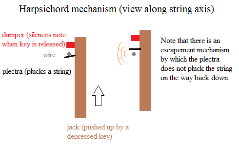
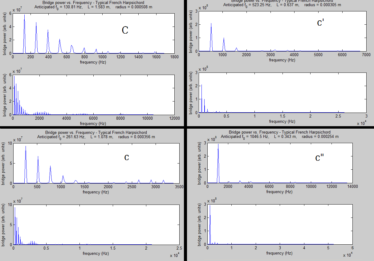
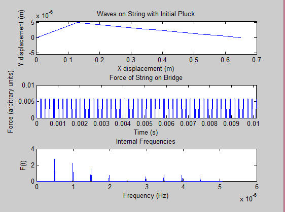
Begin with the equations for the fundamental frequency  of a vibrating string (which defines the note sounded; the quality of the sound is dependent on the strength of specific higher harmonics that also sound):

where  is string length,  is tension, and  is the total mass of the string (Vibrating String). More useful to us is the string’s volumetric mass density  :

where  is the (very small) radius of the wire. These equations can be combined to give:

Armed with an expression for tension containing only known values, the simulations can be run. Note that length, density, and radii data can be found in the bibliography (Di Veroli)(Rose)(Metals and Alloys)(Beebe).

Results

Using the following parameters (some of which are from bibliography, cited above, while others were from personal measurement), the bridge force spectra were computed:

Graphical representation of the fft’s of the four bridge force spectra computed (shown each at two different scales):

Figure 2: Force spectra for harpsichord strings given parameters above. Please click on image to view; any size other than full screen is illegible (hence why it is not full screen here).

Note that the waves in this model do not decay with time; this is a choice in the model and should not strongly effect the outcome, as the intention of the model is to simulate the harmonic frequencies immediately after the initial pluck, not the long term evolution of the system.

As the strings become shorter, the plucking point moves closer to the center of the string, changing the plucking ratio and altering the character of the sound, as indicated by a lack of abundant higher harmonics in the shorter strings (right two figures). This is in agreement with a qualitative understanding of the instrument; bass notes tend to have a more unique sound compared to the high notes.

Further, using the sound function in MATLAB to play back signals produces a very encouraging result: the sound generated purely by this computational model does, in fact, sound like a harpsichord. A further step of the project, analyzing data from the instrument itself, will tell whether or not the model is in quantitative agreement.

The next installment of this project will examine the clavichord, which has a method of sound generation almost unique among musical instruments, and hopefully will include analysis of actual harpsichord data.

Bibliography:

Beebe, “Technical Library, Stringing III: Stringing Schedules“. Accessed 4/21/2015 at http://www.hpschd.nu/index.html?nav/nav-4.html&t/welcome.html&http://www.hpschd.nu/tech/str/sched.html (see “Hemsch Double”)

Claudio Di Veroli, “Taskin Harpsichord Scalings and Stringings Revisited“. Accessed 4/21/2015 at http://harps.braybaroque.ie/Taskin_stringing2.htm

Malcolm Rose, “Wires for harpsichords, clavichords and fortepianos“. Accessed 4/20/2015 at http://www.malcolm-rose.com/Strings/strings.html

“Metals and Alloys – Densities“. The Engineering Toolbox. Accessed 4/20/2015 at http://www.engineeringtoolbox.com/metal-alloys-densities-d_50.html

“Vibrating String“. Georgia State University, Accessed 4/21/2015 at http://hyperphysics.phy-astr.gsu.edu/hbase/waves/string.html

Code

https://www.dropbox.com/s/l8f3sscmel1qdko/Kachelein_Project_Results1.m?dl=0

https://docs.google.com/a/vassar.edu/document/d/1nvyB5giUicIIiCJuKNKTwJagBlepP8J-IOQsMeMgB7Q/edit

Brownian Motion of a Drunkard

Random Unit Vector 2D Motion of a Drunkard

As shown by the standard error of the slope within slopes of the displacement squared, the Brownian Motion has a statistically significant larger displacement squared. This is before I alter the 2D code to account for more drunken chance variables. This will serve as a good baseline to see how the mean displacement changes after each variable is added or combinations of variables are tested. I chose to use brownian motion as the standard since it is purely random in every way (in my code). The direction of a step and length are always randomized. I am very pleased with how my codes came out and the visualizations they provide. I apologize for the poor quality of screenshots but they will not look this way in the final project. The top subplot is one representation of the random movement. The second is a displacement squared of one walk. The final in blue is the mean of all of the displacement squareds. The red is the best fit line with the statistics below.

This will serve as my jumping off point to compare Brownian motion of a drunkard (a gas) to a college student on the weekend with several variables and options besides just taking steps. I am curious to see how much I can alter the mean displacement squared with various variables and different weights. Unfortunately, I still need to collect more data outside of class to correctly weight the variables. I’m still catching up on other work from tech week.

After investigating the call and the put option last week, we decided to continue to investigate option or derivative trading. This time we looked at how to program binomial trees in MatLab. For a quick refresher a call option is when the owner of the asset, which can be a stock or portfolio, has the right to buy the asset at the pre-determined strike price. A put option is when the owner has the right to sell the asset at the pre-determined strike price. This means that if the asset price goes below the strike price, the put option is advantageous and makes the owner money. If the asset price goes above the strike price then the call option becomes the money making option.

So what exactly does a binomial tree look like. Below is the an example of a binomial tree when n=3 which means that past n=0 there are three distinct division. In this case at n=0 the price of the asset is 100 dollars. Binomial trees are interesting because unlike the Black-Scholes method, which was previously discussed in last weeks post, the binomial tree provides the user with a flexible way to price the option. In this example at each node the price of the asset has two alternatives it can either go up in price or down in price. Unlike the Black-Scholes model the binomial tree provides a period to period transparency in the price of the option. It is important to note that this binomial tree does not follow the same definition that a typical discrete mathematics textbook would describe a tree. This is because the binomial option pricing tree contains cycles, where as in a strict mathematically definition trees cannot contain cycles.

 (Each number is the possible price of the asset).

The binomial tree is more advantageous in pricing American options. This is because for an American option the owner at any point can exercise the option before the maturity date (when the option expires). The binomial tree works backwards to find the value of the option at T=0, when time is equal to zero. This helps determine how much one is willing to pay for the option. The binomial tree finds the difference in price between the original asset price, and the price at another discrete time interval, using the function max(K-P,0) , where K is the strike price, and P is the price of the asset at T=0. This function max(K-P,0) is used for a put option, and described more in our code.

It is important to discuss the variables the binomial tree is dependent on. It is dependent on $\sigma$ which is volatility, simply it is just the standard deviation in returns of an asset or portfolio, $r$ is risk neutral interest rate, $u$ and $d$ are percentages the asset either goes up or down at each stage of the tree. The formula for backwards induction to find the original value of the asset is…

(1)  

where $V_u$ is the upper price at a discrete stage, and $V_d$ is the lower price at a discrete stage. A discrete stage meaning n=1,2… We know need to look at what p is, well p simulates the geometric Brownian motion of the underlying stock or asset with parameters $r$ and $\sigma$. p is given by the equation below:

(2)  

We have finished the pricing of an American put option for a binomial tree when n=3. And plan on continuing to work on the code for the option pricing method to work for an arbitrary number for n, and hope to have completed by our next post.

The past week has been spent turning the basic ferromagnetic spin model (isingtest.m) created last week into a model of a basic financial system. In the ferromagnetic model, the spins of constituent atoms were represented by discrete spin values of 1 or -1. In this model, we will use the analogous atoms to represent agents in a market. This market will be based on any arbitrary good or stock, and like the ferromagnetic model, adjacent “agents” will be able to share information and influence each other. Here, the tendency for atoms to align with adjacent atoms represents a tendency of financial agents that work close to each other to use the same ideas.

In this model, a spin value of 1 signifies that an agent is currently buying the good or stock, whereas the value of -1 signifies that the agent is currently selling it. The market is governed by two rules:

1. The first rule is analogous to the ferromagnetic model: adjacent actors influence each other strongly.
2. The second rule introduces an idea analogous to a heat bath. This rule states that the agents in the minority group have a special kind of knowledge, so all agents in the market will want to be part of that minority group.

In order to initialize this market, we create a grid to store whether or not each agent is a buyer or seller. We initially assigned the majority of agents to be buyers, represented as white pixels. The sellers are interspersed as blocks throughout the market, represented by the black pixels. Below is an example of what an initial market might look like:

From here, our monte carlo method cycles through every agent in the market, using its position relative to its neighbors as well as an overall market trend to calculate the “field” that pushes it toward one strategy or another. After every iteration, the display of the grid was altered accordingly. The equation for this field is below:

(3)  

The first term in the expression is analogous to the spin alignments, whereas the second term is representative to the individual agent’s view of the whole market. The value C corresponds to whether an agent will be a “fundamentalist(C=1)” or a “chartist(C=-1).” If the agent is a fundamentalist, it means that he or she will be likely to follow the rule that it is best to try to get into the minority, making the second term negative and pushing it against the first term. If the agent is a “chartist,” it means that he or she is content with being in the majority, and the sign of the second term is the same as the first. Whether or not the agent is a fundamentalist or a chartist is determined by whether or not choosing this strategy will increase the energy, or risk, of the system, which would improve the likelihood of making money. This probability of an agent changing his or her identity is determined with:

(4)  

Then, the probability of an agent remaining/becoming a buyer is given by:

(5)  

(6)  

The second term is the probability that the agent will remain/become a seller. A random number is generated by the monte carlo method and compared to the probability, deciding which strategy the agent in question will use at the current time. Once the code has cycled through every agent in the market, it will update the grid displaying the identity of each agent’s strategy at the given time. The average value of all of the strategies in the market is then taken, as it is representative of the price of the good or the stock. A positive average represents a positive trend in price, because there are more people that want to buy than sell. The opposite is true as well, as a negative average means that there is a surplus of sellers. Taking this average and subtracting from it the average of the last iteration gives use the change in price, or return, created by a shift in the market. An example is displayed below, plotting this average vs. time:

The periods of extreme return in a negative or positive direction correspond to a market configuration where there are large groups of buyers grouped together and large groups of sellers grouped together as shown below:

Conversely, when the returns stay near 0, it is because there is no real trend in the market and it is more turbulent, as such:

Finally, another way to represent this trend is to show the difference between fundamentalists in the market compared with chartists in the market. This difference is displayed below, and it is possible to see that when there is a more extreme difference, there are more extreme changes in the return.

For our final part of this project, we will try to use the autocorrelation function to characterize the volatility of the good over time. We will also try to add another strategy option, as well as possibly exploring a 3 dimensional system. The code for this part is “TwoStrategyMarketModel.m”

Link to Code:

https://drive.google.com/folderview?id=0B01Mp3IqoCvhflF5azV4bHY2V0c3Vks0VXVyQkIxcnR4RmFaNDhVWEQtZGZSR2t6V2VWOHc&usp=sharing

The files are under the name: BinomialTreeNThree.m and TwoMarketStrategyModel.m

Here is the code for our modeled guitar string and the resulting force on the bridge.  This force oscillates with time, similar to the frequency of the sound waves that the instrument produces.  We were able to find the base and overtone frequencies using the fast fourier transform function in MatLab, however our scaling is off for graphing purposes.  However, we know our data is correct because we plucked the string at a distance (B=1/5) of the total length of the string which resulted in our fourier transform missing a 5th peak.  For future testing, we hope to record a physical string with similar variables to the one in our code, import the sound file to MatLab, analyze the frequencies, and compare it to the results of the modeled string.

——————————————————————————————————————————————

Link to code:

https://docs.google.com/document/d/1vNhrcuUVjmwfNM8raGKmyKAl0Z19bFR8c7rikb9tI1w/edit?usp=sharing

close all
clear all
%%%GUITAR STRING%%%

%% Initialize Variables
L=.65; %Length of string (m)
T=149; %Tension of string (N)
c=320; %Velocity of wave (m/s)
dx=.065; %Distance step
dt=0.00001015625; %time step (s)
r=1; %constant in oscillation calculation equation
Amp=.000005; %Amplitude of pluck (m)
Lpluck=.13; %Length of pluck spot (m)
B=Lpluck/L; %pluck position on string (m)
M=[0]; %Array for y vaules
runtime=1000;

%% Builds initial pluck array
for i=dx:dx:Lpluck
y=i*Amp/Lpluck;
M=[M,y];
end

for i=(Lpluck+dx):dx:L
y=(i-L)*(-Amp/(L-Lpluck));
M=[M,y];
end

%% Build X-aixs
x_axis=[];

for i=0:dx:L
x_axis=[x_axis,i];
end

%% Initialize Loop variables

ynew=zeros(1,length(M));
ycurrent=zeros(1,length(M));
yold=zeros(1,length(M));
ycurrent=M;
yold=M;

F=[];
N=[];

%% Animation Loop (String Oscillations)

for n=1:runtime

for i=2:length(M)-1
ynew(i)=2*(1-r^2)*ycurrent(i)-yold(i)+(r^2)*(ycurrent(i+1)+ycurrent(i-1));
end

f=T*(ynew(2)-ynew(1))/dx;
F=[F,f];

N=[N,(n*dt)];

yold=ycurrent;
ycurrent=ynew;

subplot(3,1,1)
plot(x_axis,ynew)
axis([0,0.7,-Amp*1.1,Amp*1.1])
title(‘Waves on String with Initial Pluck’);
xlabel(‘X displacement (m)’);
ylabel(‘Y displacement (m)’);

subplot(3,1,2)
plot(N,F)
axis([0,runtime*dt,0,0.01])
title(‘Force of String on Bridge’)
xlabel(‘Time (s)’)
ylabel(‘Force (arbitrary units)’)

pause(0.000001)
end

%% Tension/Frequency

FFT=fft(F);

FTscale=2^nextpow2(runtime);
f=dt/2*linspace(0,1,FTscale/2+1);

subplot(3,1,3)
plot(f,(2*abs(FFT(1:FTscale/2+1))))
title(‘Internal Frequencies’)
xlabel(‘Frequency (Hz)’)
ylabel(‘F(t)’)

%need to fix scale on FT

As of 4/13, I have yet to finish hacking and reassembling all of the equipment in my laboratory to take my own EMG (electromyography) data. As a refresher, an EMG is a means of measuring nerve activity by analyzing voltage changes in muscles either on the surface of the skin or subcutaneously. However, I believe that I should be able to complete the relevant assembly of the EMG kit prior to the end of the project.

That being said, I have completed the initial version of my data analysis code to be implemented in this project, as well as in my thesis. This version uses two data set inputs, a raw EMG signal, and a corresponding time vector. In addition, the code requires the sampling frequency. Beyond this, the experimenter has to set noise and contraction thresholds. The noise threshold serves the dual purpose of compensating for any noise not already dealt with in the Fourier transform, as well as setting the region below which the robot will relax and return to the rest state. The contraction threshold, determined by the relative magnitude of successive peaks to a standard strained peak determined immediately following the transform process.

The two Fourier transforms performed on the raw data, forward and back, allow the code to eliminate the most significant predictable sources of noise, that if left ignored, would render any analysis worthless. The three largest sources accounted for currently are movement artifacts, electrical artifacts, and electric noise. The first two noise signals are generated as a byproduct of the EMG process, mostly existing below 20 Hz. Most electric devices emit strong interference at 60 Hz. Following the forward transform, these frequencies are negated and zeroed, then back transformed to create a rectified, useable signal for later analysis.

The code is meant to reliably extract the peak amplitudes and cycle durations of up to two contractions by binning the raw EMG data into smaller datasets that are then analyzed. The reasons for this are that it makes coding less difficult as well as opening up the possibility of a quasi-continuous computation. By chopping  the data into bins and analyzing them separately, the code can process data quickly after the signals are created, which in a living subject, corresponds to continuous motion of the prosthesis. In the picture below, the initial analysis code is represented as a flowchart.

Additionally, I have found a raw sample EMG data set with a time vector, which if needed, can serve as the data for this project. This was available on a public domain, the link to which is below the figure of a raw EMG signal below and in the corresponding google drive document attached to this submission.

http://physionet.org/physiobank/database/emgdb/

Further work will include improving my code such that it is more independent of the data inputted, more modular, and generally faster/more efficient. Additionally, I have yet to comment on the code, which will be another component of this project. I expect for the final data to have improved my code and run analysis on either data that I have taken, or if I cannot get my experiment assembled and working to a reasonable extent, the sample EMG that was available online.

Relevant files can be found here:

https://drive.google.com/drive/u/0/#folders/0B0K4JjJfDy1ffkR4eEZaMzlxb0xvTjRjWDBIUm9iVzZuRmVyeG1aM0RhWHMxcVB6RXZDUFk