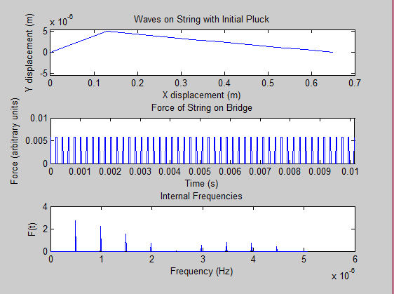
Here is the code for our modeled guitar string and the resulting force on the bridge.  This force oscillates with time, similar to the frequency of the sound waves that the instrument produces.  We were able to find the base and overtone frequencies using the fast fourier transform function in MatLab, however our scaling is off for graphing purposes.  However, we know our data is correct because we plucked the string at a distance (B=1/5) of the total length of the string which resulted in our fourier transform missing a 5th peak.  For future testing, we hope to record a physical string with similar variables to the one in our code, import the sound file to MatLab, analyze the frequencies, and compare it to the results of the modeled string.

 

 

——————————————————————————————————————————————

Link to code:

https://docs.google.com/document/d/1vNhrcuUVjmwfNM8raGKmyKAl0Z19bFR8c7rikb9tI1w/edit?usp=sharing

 

 

close all
clear all
%%%GUITAR STRING%%%

%% Initialize Variables
L=.65; %Length of string (m)
T=149; %Tension of string (N)
c=320; %Velocity of wave (m/s)
dx=.065; %Distance step
dt=0.00001015625; %time step (s)
r=1; %constant in oscillation calculation equation
Amp=.000005; %Amplitude of pluck (m)
Lpluck=.13; %Length of pluck spot (m)
B=Lpluck/L; %pluck position on string (m)
M=[0]; %Array for y vaules
runtime=1000;

%% Builds initial pluck array
for i=dx:dx:Lpluck
y=i*Amp/Lpluck;
M=[M,y];
end

for i=(Lpluck+dx):dx:L
y=(i-L)*(-Amp/(L-Lpluck));
M=[M,y];
end

%% Build X-aixs
x_axis=[];

for i=0:dx:L
x_axis=[x_axis,i];
end

%% Initialize Loop variables

ynew=zeros(1,length(M));
ycurrent=zeros(1,length(M));
yold=zeros(1,length(M));
ycurrent=M;
yold=M;

F=[];
N=[];

%% Animation Loop (String Oscillations)

for n=1:runtime

for i=2:length(M)-1
ynew(i)=2*(1-r^2)*ycurrent(i)-yold(i)+(r^2)*(ycurrent(i+1)+ycurrent(i-1));
end

f=T*(ynew(2)-ynew(1))/dx;
F=[F,f];

N=[N,(n*dt)];

yold=ycurrent;
ycurrent=ynew;

subplot(3,1,1)
plot(x_axis,ynew)
axis([0,0.7,-Amp*1.1,Amp*1.1])
title(‘Waves on String with Initial Pluck’);
xlabel(‘X displacement (m)’);
ylabel(‘Y displacement (m)’);

subplot(3,1,2)
plot(N,F)
axis([0,runtime*dt,0,0.01])
title(‘Force of String on Bridge’)
xlabel(‘Time (s)’)
ylabel(‘Force (arbitrary units)’)

pause(0.000001)
end

%% Tension/Frequency

FFT=fft(F);

FTscale=2^nextpow2(runtime);
f=dt/2*linspace(0,1,FTscale/2+1);

subplot(3,1,3)
plot(f,(2*abs(FFT(1:FTscale/2+1))))
title(‘Internal Frequencies’)
xlabel(‘Frequency (Hz)’)
ylabel(‘F(t)’)

%need to fix scale on FT