After investigating the call and the put option last week, we decided to continue to investigate option or derivative trading. This time we looked at how to program binomial trees in MatLab. For a quick refresher a call option is when the owner of the asset, which can be a stock or portfolio, has the right to buy the asset at the pre-determined strike price. A put option is when the owner has the right to sell the asset at the pre-determined strike price. This means that if the asset price goes below the strike price, the put option is advantageous and makes the owner money. If the asset price goes above the strike price then the call option becomes the money making option.

So what exactly does a binomial tree look like. Below is the an example of a binomial tree when n=3 which means that past n=0 there are three distinct division. In this case at n=0 the price of the asset is 100 dollars. Binomial trees are interesting because unlike the Black-Scholes method, which was previously discussed in last weeks post, the binomial tree provides the user with a flexible way to price the option. In this example at each node the price of the asset has two alternatives it can either go up in price or down in price. Unlike the Black-Scholes model the binomial tree provides a period to period transparency in the price of the option. It is important to note that this binomial tree does not follow the same definition that a typical discrete mathematics textbook would describe a tree. This is because the binomial option pricing tree contains cycles, where as in a strict mathematically definition trees cannot contain cycles.

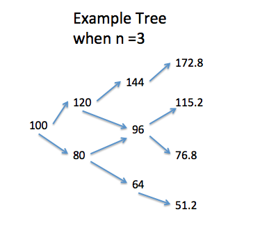
 (Each number is the possible price of the asset).

The binomial tree is more advantageous in pricing American options. This is because for an American option the owner at any point can exercise the option before the maturity date (when the option expires). The binomial tree works backwards to find the value of the option at T=0, when time is equal to zero. This helps determine how much one is willing to pay for the option. The binomial tree finds the difference in price between the original asset price, and the price at another discrete time interval, using the function max(K-P,0) , where K is the strike price, and P is the price of the asset at T=0. This function max(K-P,0) is used for a put option, and described more in our code.

 

It is important to discuss the variables the binomial tree is dependent on. It is dependent on $\sigma$ which is volatility, simply it is just the standard deviation in returns of an asset or portfolio, $r$ is risk neutral interest rate, $u$ and $d$ are percentages the asset either goes up or down at each stage of the tree. The formula for backwards induction to find the original value of the asset is…

(1)  

where $V_u$ is the upper price at a discrete stage, and $V_d$ is the lower price at a discrete stage. A discrete stage meaning n=1,2… We know need to look at what p is, well p simulates the geometric Brownian motion of the underlying stock or asset with parameters $r$ and $\sigma$. p is given by the equation below:

(2)  

We have finished the pricing of an American put option for a binomial tree when n=3. And plan on continuing to work on the code for the option pricing method to work for an arbitrary number for n, and hope to have completed by our next post.

The past week has been spent turning the basic ferromagnetic spin model (isingtest.m) created last week into a model of a basic financial system. In the ferromagnetic model, the spins of constituent atoms were represented by discrete spin values of 1 or -1. In this model, we will use the analogous atoms to represent agents in a market. This market will be based on any arbitrary good or stock, and like the ferromagnetic model, adjacent “agents” will be able to share information and influence each other. Here, the tendency for atoms to align with adjacent atoms represents a tendency of financial agents that work close to each other to use the same ideas.

In this model, a spin value of 1 signifies that an agent is currently buying the good or stock, whereas the value of -1 signifies that the agent is currently selling it. The market is governed by two rules:

1. The first rule is analogous to the ferromagnetic model: adjacent actors influence each other strongly.
2. The second rule introduces an idea analogous to a heat bath. This rule states that the agents in the minority group have a special kind of knowledge, so all agents in the market will want to be part of that minority group.

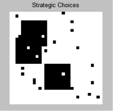
In order to initialize this market, we create a grid to store whether or not each agent is a buyer or seller. We initially assigned the majority of agents to be buyers, represented as white pixels. The sellers are interspersed as blocks throughout the market, represented by the black pixels. Below is an example of what an initial market might look like:

 

From here, our monte carlo method cycles through every agent in the market, using its position relative to its neighbors as well as an overall market trend to calculate the “field” that pushes it toward one strategy or another. After every iteration, the display of the grid was altered accordingly. The equation for this field is below:

(3)  

The first term in the expression is analogous to the spin alignments, whereas the second term is representative to the individual agent’s view of the whole market. The value C corresponds to whether an agent will be a “fundamentalist(C=1)” or a “chartist(C=-1).” If the agent is a fundamentalist, it means that he or she will be likely to follow the rule that it is best to try to get into the minority, making the second term negative and pushing it against the first term. If the agent is a “chartist,” it means that he or she is content with being in the majority, and the sign of the second term is the same as the first. Whether or not the agent is a fundamentalist or a chartist is determined by whether or not choosing this strategy will increase the energy, or risk, of the system, which would improve the likelihood of making money. This probability of an agent changing his or her identity is determined with:

(4)  

Then, the probability of an agent remaining/becoming a buyer is given by:

(5)  

(6)  

The second term is the probability that the agent will remain/become a seller. A random number is generated by the monte carlo method and compared to the probability, deciding which strategy the agent in question will use at the current time. Once the code has cycled through every agent in the market, it will update the grid displaying the identity of each agent’s strategy at the given time. The average value of all of the strategies in the market is then taken, as it is representative of the price of the good or the stock. A positive average represents a positive trend in price, because there are more people that want to buy than sell. The opposite is true as well, as a negative average means that there is a surplus of sellers. Taking this average and subtracting from it the average of the last iteration gives use the change in price, or return, created by a shift in the market. An example is displayed below, plotting this average vs. time:

 

 

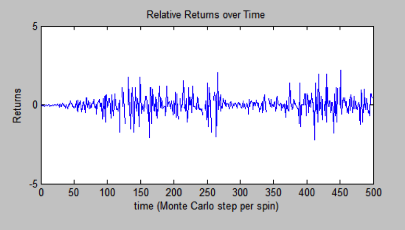
The periods of extreme return in a negative or positive direction correspond to a market configuration where there are large groups of buyers grouped together and large groups of sellers grouped together as shown below:

 

Conversely, when the returns stay near 0, it is because there is no real trend in the market and it is more turbulent, as such:

 

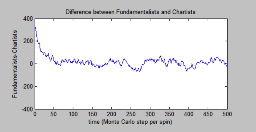
Finally, another way to represent this trend is to show the difference between fundamentalists in the market compared with chartists in the market. This difference is displayed below, and it is possible to see that when there is a more extreme difference, there are more extreme changes in the return.

 

For our final part of this project, we will try to use the autocorrelation function to characterize the volatility of the good over time. We will also try to add another strategy option, as well as possibly exploring a 3 dimensional system. The code for this part is “TwoStrategyMarketModel.m”

Link to Code:

https://drive.google.com/folderview?id=0B01Mp3IqoCvhflF5azV4bHY2V0c3Vks0VXVyQkIxcnR4RmFaNDhVWEQtZGZSR2t6V2VWOHc&usp=sharing

The files are under the name: BinomialTreeNThree.m and TwoMarketStrategyModel.m