Molecular Dynamics Project Conclusions

Molecular Dynamics Project Summary

Sushant Mahat and Mohammed Abdelaziz

Over the last few weeks, we have been working on a computational project on molecular dynamics. This post below summarizes the details of this project, and the overall goals we achieved.


Initial Goals and Motivations:

We wanted to do an experiment in molecular dynamics as it connects to several things we have studied in our previous physics classes. We used our knowledge on Newton’s second law which we learned in classical mechanics; we used Boltzmann’s distribution and the concepts of temperature from thermodynamics and statistical mechanics; and we used the Lennard-Jones potential which has its root in quantum mechanics. All these features made simulating  molecular dynamics an attractive, challenging, and a very educational project.

We had several goals when we started this project. We wanted to be able to simulate a 2-D gas system, and be able to study several of its properties like temperature, energies, speed distributions, and visualization at equilibrium. We then wanted to build up on this system to make it into a 3-D system. We were also thinking about making it possible to increase the temperature of the system and observe how long it takes to come back to equilibrium. This was supposed to be a simulation of periodic heating of gas particles with a laser beam.


Goals We Completed

Due to time constraints, we were unable to fulfill some of our initial goals. However, we were able to finish most of the goals. The goals we met for this project include:

  1. Simulating the motion of a dilute sample of gaseous Argon atoms in two dimensions.
  2. Calculating the mean velocities of each atom and plotting their speed distribution in each simulation.
  3. Determining the temperature of the sample based on initial and equilibrium speeds of each atom, which required a determination of the kinetic energies of all atoms at each time step.
  4. Comparing the calculated speed distribution with the Maxwell-Boltzmann speed distribution curve.
  5. Completing the simulation and the above calculations in three dimensions.
  6. Introduced possibility to simulate temperature change in the system.


Methods

Section 9.1 of Giordano and Nakanishi’s Computational Physics was our primary reference for this project. We used MATLAB for the simulations, dividing our code into several functions (subroutines) instead of using one script. The codes and their purposes are outlined below.


TheInitiator.m

This function initializes an evenly spaced grid in 3-D space (2-D in the old version of the program). This grid serves as the basis for the location of each atom, because we want the atoms to start at roughly the same location for each simulation. Two further steps are taken to make sure the simulations are not fully deterministic: each atom was displaced slightly from a point on this evenly spaced grid, and it was given a random velocity (within some limits) in each dimension. This function also allows an option to have different limits of the initial random velocity which can produce an effect similar to starting with gas particles with different temperature.


TheEnforcer.m

This function calculates the force on each atom due to every other atom, based on the Lennard-Jones potential, which is ineffective at large distances, attractive at moderate distances, and repulsive at very short distances. This calculation takes exponentially longer for additional particles, because each particle interacts with each other particle.


TheUpdater.m

This function uses the forces from the previous function and each particle’s positions to calculate each particle’s position and velocity at the next time step. It feeds these positions back into TheEnforcer.m and iterates until the positions and velocities of each particle for each time step are calculated. This function also enforces the periodic boundary conditions (that a particle leaving one side of the “box” comes back through the other side, with its velocity unaffected). Particles that are closer to each other through these boundary conditions than they appear must interact as though they were at this close distance. To clarify this, consider a one-dimensional system, ranging from x=0 to x=10. Two particles at x=1 and x=9 should interact as if they are 2 units apart, not 8 units apart. Implementing this system properly was one of the most difficult tasks we faced.


SpeedDist.m

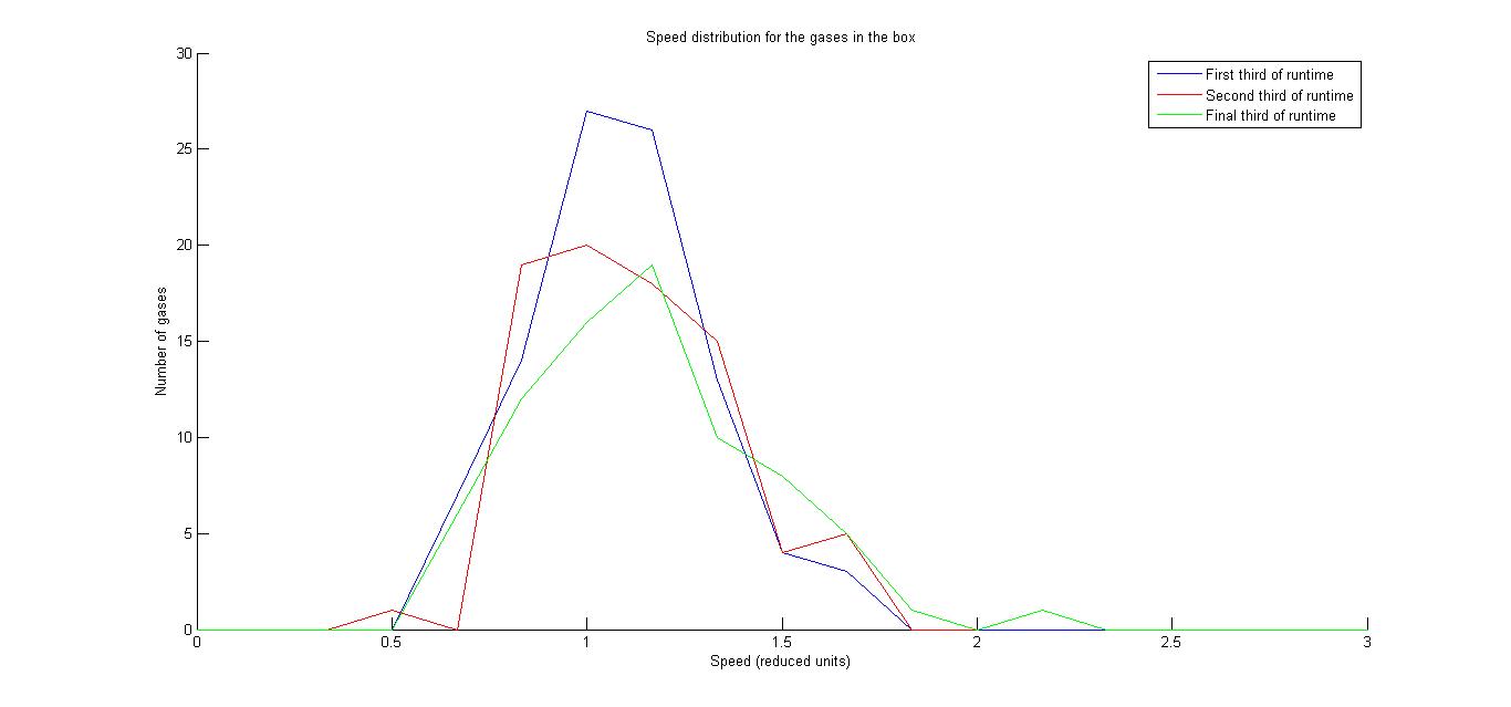
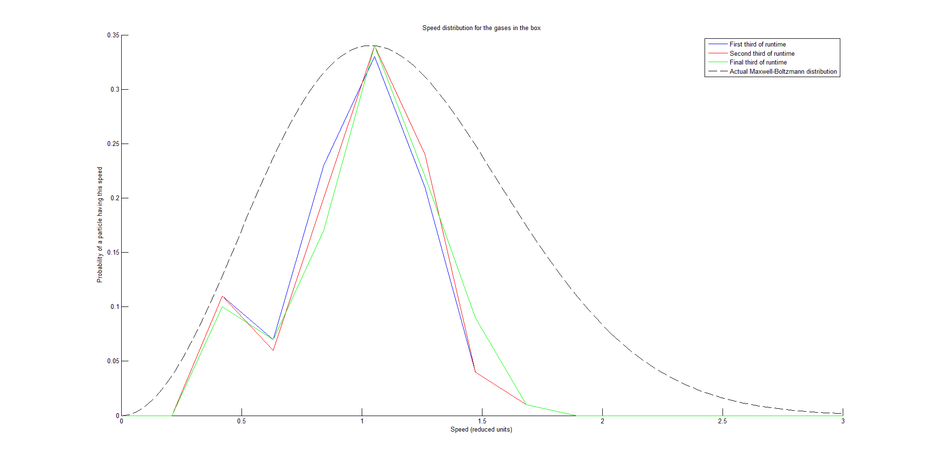
This function takes in each velocity component of each particle at each time step, and first calculates a speed for each particle at each time step. It plots three speed distribution curves by averaging each particle’s speed over each third of the runtime, placing these speeds into bins, and plotting a histogram that is visualized as a curve. The function is configurable to plot any integer D speed distribution curves by averaging each particle’s speed over each 1/D of the runtime instead, but D = 3 effectively showed that the system had reached equilibrium (signified by when two successive speed distribution curves are fairly similar).

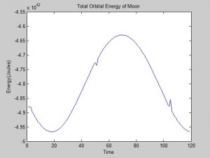
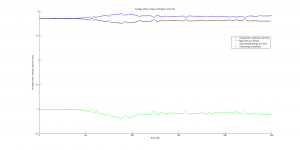
This function also plots the kinetic, potential, and total energy averaged for all particles at each time step in the simulation. The kinetic energy was needed to calculate temperature, since the product of Boltzmann’s constant and the system’s temperature is equal to the average kinetic energy of all particles in the system.


MainBody.m

This script simply initializes the spatial dimensions of the system and how many atoms will be simulated. This is the code that is directly run by the user to visualize the simulation and look at the speed distributions and energies.

All of these MATLAB files can be found in this Google Drive folder.


Results

We succeeded in producing visualizations of the Argon atoms in two and three dimensions. Even with 100 atoms, the script does not take more than thirty seconds to run, so more particles could feasibly be simulated. Additionally, our speed distributions matched up relatively well with the actual Maxwell-Boltzmann distributions in terms of horizontal location (this shows that our determination of temperature was accurate, since this is what affects the horizontal position of the peak (most common particle speed). However, our generated speed distributions were more narrow than the Maxwell-Boltzmann distribution. It is possible that they could be widened by decreasing the density of the atoms (simulating fewer particles or making the dimensions of the “box” bigger). It is also possible that increasing the maximum initial velocity would increase the width of the speed distribution, since it would give each particle a wider range of initial velocities to have.

We were mostly satisfied with our energy plots; they showed a fairly constant total energy, which we expect (it is not completely constant because the total energy is calculated from averages of kinetic and potential energy of all particles). Kinetic and potential energies became steady as the system reached equilibrium, which takes longer for lower gas densities.

One example of a speed distribution plot (click for full-size):

speedDistImage

One example of an energy plot (click for full-size):

energies


Conclusion and Future Potential

Based on the Boltzmann’s distribution plots of our data, we are fairly confident that our simulation is useful at approximating systems of gas molecules. The fact that the total energy of the system remains around a fixed value is also promising. However, the fluctuations in the total energy when the particles start interacting is still not ideal.

One limitation of our problem would be that the system destabilizes when the initial density of our gas molecules are very high. This is a direct result of the steep increase in the Lennard-Jones potential at low distances between particles.

We want our readers to see this code as a work in progress rather than a complete program. The program still has a lot of unrealized potential. For example, the energy graph produced by the simulation for cases with different initial velocity limits could potentially be used to calculate time taken by a system with gases of different temperature to equilibrate. Similarly, with some changes to the initiator and the enforcer function, the program could also be used to simulate a collection of different gases as opposed to a single type of gas molecule. Although we were unable to simulate it, increasing the density and lowering the initial velocity should also make it possible for future users to simulate materials in solid and liquid phases. Since the program already has method to change temperature built into it, some changes could be made to make these temperature changes periodic. This could potentially be used to simulate a laser beam heating the gas particles.

Overall, we are very satisfied with the progress we were able to make throughout the semester. Apart from learning a great deal about different physical concepts, we also developed a deeper appreciation and knowledge of computational approaches towards studying physical systems. We also think that we have developed  a fair understanding of the limitations and the potential of the computational tools available to us, and we are confident that this project has prepared us for many more simulations that we are likely to encounter in our careers as physicists.         

Matteo & Nadav: Final Conclusions

For our project we decided to model the perturbations of Earth’s orbit caused by Jupiter. We chose to study the effects of Jupiter because it is the only mass nearly comparable to the sun (about 0.1%). We started with a routine that modeled a single planet orbiting a fixed Sun, and built up to a true three body simulation with the Earth, Sun, and Jupiter bound gravitationally.

Our end goal was to write a three body simulation for the planets because we planned to observe the effects of an increased Jupiter mass on Earth’s orbit. At a certain point the “fixed-Sun” model becomes an unphysical approximation. Three body problems are nearly impossible to solve besides restricted problems, but quite possible to observe computationally.

Routine I: Planet Orbit

Our first model just contained a single planet orbiting around the sun. Mathematically, this model only relied on the inverse square law of gravity to relate the two bodies. Since we know from the physical system that sun is far more massive than any of the planets, we know that they have a negligible effect on the sun’s orbit. Because of this we simply fixed the sun at the origin of our system, and only modeled the movement of the planet around it.

We chose the Euler Cromer method as our primary tool because the orbit of a planet is an oscillatory motion and energy needs to be conserved over each period. This is comparable to the pendulum problems from earlier in the semester where we ran into the same issue. With the Euler method energy is added each period, so we demonstrated here that the Euler-Cromer method conserves energy with each orbit.

earthEC       earthE

Euler Cromer                                                         Euler

Thus, the only thing affecting each orbit is actually the initial conditions, we are essentially approximating all of the orbits except mercury as circular because their eccentricities are very close to zero. Due to this nearly circular motion, the gravitational force is equivalent to the centrifugal force of a body in uniform circular motion and we are able to calculate the initial velocity for the planet when it starts at a distance of its semi-major axis from the sun. We will observe circular motion unless the initial velocity is wrong.

Routine II: Jupiter-Earth

 Already having completed a foundational program for a gravitationally bound singular planet simulation, it was not much of a reach to add in a second planet for our second routine. The exact same physical equations were used and we continued using the Euler-Cromer approximation method. Initially, once Earth and Jupiter are related gravitationally, we observe no noticeable difference in the Earth’s orbit, which matches our physical observations. This program is very useful however because it allows us to adjust Jupiter’s mass in order to observe how the Earth’s orbit perturbs without affecting the sun’s motion. While this was very useful as an initial exploration into the perturbations of Earth’s orbit caused by Jupiter, it was not complete because it still didn’t take into account the motion of the Sun when Jupiter’s mass was very large. This was the goal of our next routine.

Jupiter Earth 1Jupiter Earth 500


Routine III: Three-Body

The difference between the three-body routine and the earth-jupiter routine is that we no longer fix the sun in place and instead calculate the effects of Jupiter and Earth on its motion. We also made several changes to the initial conditions to make the model work, such as changing the origin to be the center of mass of the system and giving the sun an initial velocity so that the center of mass does not drift. We also set it so that the initial velocity of sun changes with increase in the mass of Jupiter in order to maintain these conditions.

3body 100xjupiter mass3body sensitive to change in initial condition2

Observations:

These simulations demonstrated that the Earth’s orbit is very stable even up to many times the current mass of Jupiter (as would be expected from observational evidence).

Upon observing the effects of changes in Jupiter’s mass for this system, we were able to conclude that the final three-body system becomes chaotic at sufficient Jupiter masses. Small changes in Jupiter’s mass caused entirely distinct orbits to form. In many of these systems, the motion appeared completely random, sometimes resulting in the Earth’s ejection from the system. Just like the pendulum, below a certain driving force the pendulum’s motion was still predictable, and above a certain force the motion became chaotic.

This threshold for chaotic motion was clearly demonstrated when the mass of Jupiter approaches the sun’s mass (x1000). The system starts to look very much like a binary star system around a center of mass. In this scenario earth’s orbit is VERY unstable and chaotic, completely unpredictable, and extremely sensitive to initial conditions.  When Jupiter’s mass is sufficiently small to never directly interact with earth (AKA never crosses or comes near the path of the sun’s motion) then the motion of Earth is not chaotic.


To download our code, please click the following image:

matlabFile

Final Project Conclusions – Kachelein

Introduction

Each musical instrument has its own characteristic sound due to the contributions of different harmonic intervals above the fundamental frequency. The relative strengths of these harmonics are due to the mechanism of sound production and transmission of the instrument. For my project, I modeled the sound generation of two musical instruments, the harpsichord and clavichord. Building upon content in the class text (Giordano and Nakanishi, specifically chapters 6 and 11), I simulated the plucking action of the harpsichord for different values of several input parameters, compared computational results to data from a real instrument, and designed and executed a computational model for the clavichord.

Mathematical Background

For both instruments, the initial wavefronts evolved in time via

  \\y(i,n+1)=2[1-r^2]y(i,n)-y(i,n-1)+r^2 [y(i+1,n)+y(i-1,n)]

where i is the spacial index of the wire’s height y, n is the temporal index,  r=c\Delta t/\Delta x = 1 , Δx is the spacial step size, and Δt is the time step size. The parameter c is the speed of the wave on the string, and relied on several parameters of the string via

  c = \frac{1}{R}\sqrt{\frac{T}{\pi\rho}}

where T is the tension on the string, R is the radius of the string, and ρ is the density of the string material. The final key equation needed is for the tension:

  T = \pi\rho(2 L R f_0)^2

where L is the length of the string and f_0 is the fundamental frequency of the note desired. It should also be noted how to calculate the force of the string on the bridge (where sound is transmitted to the soundboard and then the air) using eq. 11.4:

F_{\text{bridge}}=T\frac{y(2,n)-y(1,n)}{\Delta x}

Harpsichord

The computational model for the harpsichord was identical to that of a guitar; both are plucked string instruments that function in essentially the same way. Therefore, the initial wavefront was triangular. The plucking ratio β, a parameter used to set up the wavefront, proved to have the most effect on the frequencies generated (see figure 1). This can be explained by the formation of an antinode at the plucking point; if the string is plucked near its very edge, high frequencies will be present in the signal, as these frequencies result from standing waves on the string with much smaller wavelengths than the fundamental frequency. Because c is constant, these waves will have a high frequency contribution to the overall sound (recall that f = \frac{c}{\lambda}). Interestingly, the formation of an antinode at the plucking point prohibits frequencies that require a node at that point; for instance, a string plucked in the middle (β = 0.5) will only contain the fundamental frequency, the third harmonic, the fifth harmonic, etc., as seen in figure 1.

Beta_varied_Image

Figure 1 (click to expand): Variations in acoustic spectrum due to different plucking ratios. The strings here had a fundamental frequency of 261.63 Hz (middle c). Note that β > 0.5 simply means that the plucking point was not on the same half of the string as the bridge (sound transmission point). For instance, a plucking ratio of 0.75 is the same as one of 0.25 due to the symmetry of the string and has no bearing on the acoustic spectrum.

Changing other parameters (R, L, and plucking amplitude) had no effect on the relative strengths of the frequencies in the spectrum, assuming that all other independent variables were held constant. This may indicate a weakness in the model, as builders avoid deviating from tried-and-true ratios to avoid producing unpleasant sounds (as well as to avoid combinations of R and L that would require tensions that break strings).

The importance of β in producing a particular acoustic spectrum is evident in instrument construction. Harpsichords often have two plucking distances per note from which the player can choose, depending on the desired tonal effect.

After I developed a computational model, I compared results to recordings of individual notes from a real harpsichord. The .wav files used were part of a freely available sound bank of an instrument, designed to be used without intent for profit in musical instrument emulation software (Bricet & Garet 2007). Thus, the quality of the samples is high. Figure 2 compares the sound of the real instrument with that of the model; though the latter is clearly digitally generated, the sound produced is at least qualitatively similar to the physical system it models.

Figure 2: Qualitative comparison of actual data vs. model-generated data, link here (Youtube videos do not come through for all users).

Quantitative analysis of the accuracy of the model vs. the physical data was not performed; this would have been essentially impossible without accurately knowing the plucking ratios built into the instrument that was recorded (there are no standards for β, which vary from one instrument to another and which are different note by note within the same instrument). However, I did plot generated acoustic spectra along side physical spectra in order to visually compare the model to the system (see figures 3 through 6). Though the relative strengths of the harmonic frequencies often mismatched, the model was very accurate in predicting which frequencies would be represented in a signal.

C2Image_small2 C2Image2

Figures 3 (at left) and  (right): Model (blue) and physical data (red) acoustic spectra for the note one octave below middle c (f_0 = 130.81 Hz). Figure 4 is simply a restriction of the data plotted in figure 3 to lower frequencies only. Some frequencies’ relative strengths matched well (e.g. second and third harmonics), while others were badly mismatched (e.g. first and fourth harmonics).

c5Image_smallestc5Image2

Figures 5 and 6: Similar to figures 3 and 4, but for the note two octaves above middle c (f_0 = 1046.5 Hz).

Clavichord

The mechanism of the clavichord is unique among musical instruments. Instead of hammering, plucking, or bowing a string, the string is struck at one end by a blunt metal point (via a piano-like key). The metal point, called a “tangent,” serves as one end of the sounding portion of the string; in effect, the player directly controls the boundary conditions of the system and can even slightly adjust the tension at will. Because there is no plucking point, a new computational model needed to be implemented.

The difference between the clavichord and harpsichord required only a few changes in code. Instead of beginning the string as a triangle with a peak at the plucking point, the string began straight but with a negative slope. Upon running the program, one end of the string was raised over a length of time t_{strike}
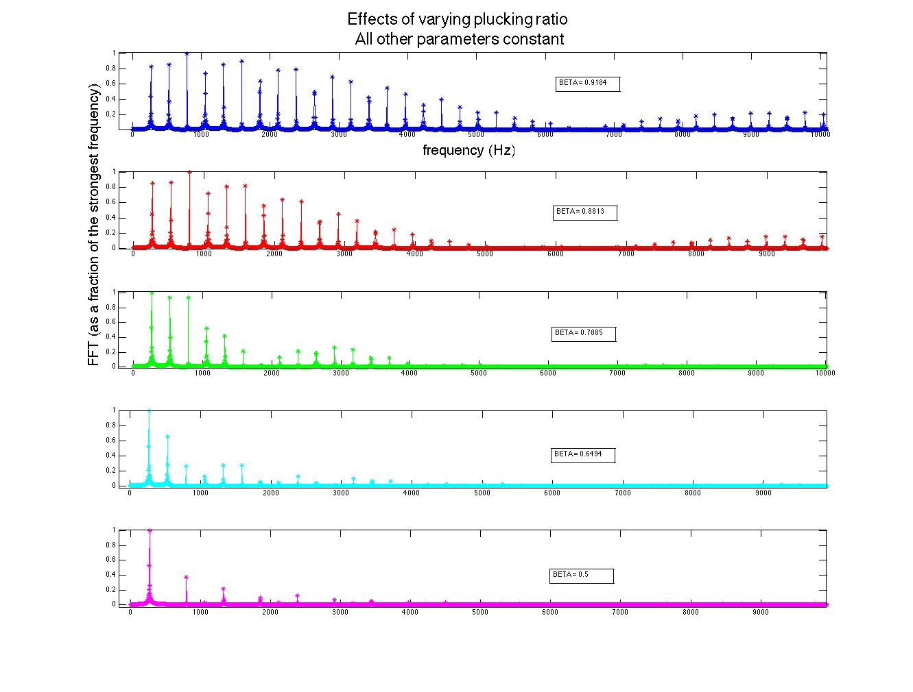
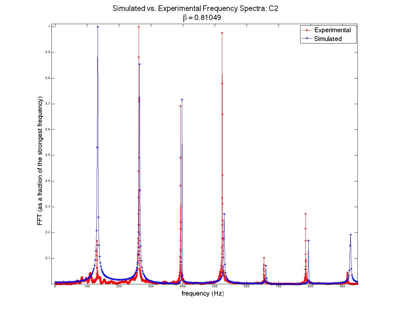
; when this time had passed, the moving end of the string became stationary, held in place for the remainder of the simulation. The time evolution of the string, the force on the bridge, and the Fourier transform (acoustic spectrum) of a note on the clavichord can be seen in figure 7.

clavichord

Figure 7Time evolution of clavichord string, bridge force, and acoustic spectrum.

Though acoustic spectra could be produced as they were for the harpsichord, these would not be illuminating, as I do not have audio recordings of individual clavichord notes with which to compare. However, due to the unrealistic sound that the model generates (not provided here), I suspect that the model, which is likely a good start, may be inadequate for several reasons. The fact that the model string starts stationary on the bridge end (see figure 7) requires many time steps to “even out.” Thus, low frequencies which are not part of the actual sound may be over-represented (note the initially strong contributions by f = 0 Hz). Second, all real clavichords have two strings per note, which may interact in subtle but significant ways that this simple model does not address. Finally, the tension in a real clavichord string changes slightly as the key is depressed, and that is not accounted for in this model.

Conclusions

Though there are issues with the models, especially the one I designed for the clavichord, all were successfully implemented and, with further refinements and more accurate input parameters (which are not possible without access to the instrument recorded), these models could be applied to instrument design. For instance, one could determine the optimal dimensions to achieve a desired tonal quality from an instrument.

In summary, I tested the validity of a given model against actual data, varied input parameters to determine effects on the model’s output, and derived a new model to describe a system that, at this early stage, seems to be reasonable if not somewhat simplistic. Beyond describing Baroque keyboard instruments, which I personally found to be an interesting topic, this project was a general exercise in research on a small scale. I started with a model or derived my own, implemented the model computationally, generated computational data, and compared the results to experimental data.

Code

https://www.dropbox.com/sh/paquzk0tml03k0j/AACz5zNErUctcIUKiJtFUesJa?dl=0

Ignore requests to sign up for a free Dropbox account; files can be downloaded without one.

Bibliography

Beebe, “Technical Library, Stringing III: Stringing Schedules“. Accessed 4/21/2015 at http://www.hpschd.nu/index.html?nav/nav-4.html&t/welcome.html&http://www.hpschd.nu/tech/str/sched.html (see “Hemsch Double”)

Bricet & Garet 2007, “Small Italian Harpsichord.” Accessed 5/11/15 at http://duphly.free.fr/en/italien.html

Claudio Di Veroli, “Taskin Harpsichord Scalings and Stringings Revisited“. Accessed 4/21/2015 at http://harps.braybaroque.ie/Taskin_stringing2.htm

Giordano N J, Nakanishi H. “Computational Physics, 2nd Edition.” 2005. Addison-Wesley. ISBN-10: 0131469908.

Malcolm Rose, “Wires for harpsichords, clavichords and fortepianos“. Accessed 4/20/2015 at http://www.malcolm-rose.com/Strings/strings.html

– MATLAB R2014b by MathWorks®

Metals and Alloys – Densities“. The Engineering Toolbox. Accessed 4/20/2015 at http://www.engineeringtoolbox.com/metal-alloys-densities-d_50.html

Vibrating String“. Georgia State University, Accessed 4/21/2015 at http://hyperphysics.phy-astr.gsu.edu/hbase/waves/string.html

Conclusion-Brian and Tewa

Outline:

1. Questions from Comments

2. Analysis of our Neural Network

3. Concluding Remarks

4. Future Plans

1. Questions from Comments:

In this section, we will be answering the questions we received from our last post.

  1. It seems that not every neuron is connected to EVERY other neuron since there are different connection pattern.
  2. When you say an energy of “-5000″ what are your units/reference point?  I am still wondering how and why the Monte Carlo Method works and how the energy state is so low for ordered systems.  This may be unrelated and somewhat random, however, why is it that entropy (disorder) in chemistry always increases and is actually considered a lower state of energy?

Every neuron in our neural network is connected to one another. The results of their connection can be found within the j-matrix; each pattern has it’s own j-matrix.  When we store multiple patterns in one system, separate J matrices are created for each pattern, but the J matrix that is used (J_total) is the element-wise average of the separate J matrices.  So, for each neural network there is only one J matrix, which describes the connections between each neuron and every other neuron.

When a pattern is greatly distorted it takes more energy to return it back to the desired pattern. However, entropy states that the greater the disorder the lower the state of energy. Our neural network is an artificial system that has no relations to entropy. Our energy state for ordered patterns is less than that of disordered patterns because that is the way our code is designed. Furthermore, our j-matrix is designed so that when we calculate the energy of stored patterns it gives us a large negative value for energy. However, when we calculate the energy of disordered patterns it gives us energies close to zero.  The energy calculated in our neural network does not have units; it’s similar to intensity where we are just concerned with the relative energy between the neurons. The Monte Carlo method simply goes through a distorted pattern and determines whether or not a neuron needs to be flipped. This decision is based on the input of one neuron from the summation of the inputs of  the other neurons within the neural network.

2. Analysis of our Neural Network:

Since our last post we have created neural networks with a larger number of patterns stored, in an attempt to study the system as it begins to fail correct memory recall.  The way we accomplished this was by building systems with more letters as stored patterns.  We had a system which stored A-C, one which stored A-D, and one that had A-F and also a lowercase letter a.  Pictures of all of the letters we used as stored patterns are shown below.

Below are the 7 stored patterns within our neural network.

input_A  input_B  input_normal_C  input_D  input_E  input_F  input_little_a

These systems (and links to their codes) are discussed below, but first a little background on the storage of many patterns in neural networks.

As explained in our previous posts, storing more patterns in a neural network causes these patterns to become more unstable: if you think of the energy energy landscape picture from our last post, the minima associated with each pattern become shallower the more patterns that are stored.  This occurs because of the averaging of all the J matrices that correspond to the individual patterns that we want to store: each new pattern distorts parts of the other patterns.  This can be seen visually in the pictures of the J matrices in our last post; the combination of A and B is much more complicated than A and B on their own.

Our textbook (Giordano and Nakanishi) talks about the limitations of how many patterns can be stored in a neural network.  The main obstacles are that 1. any patterns that are too close to each other will likely interfere, and 2. there is a theoretical limit at which the system changes and all patterns become unstable.

For 1., think of the energy landscape again, as well as the letters we use.  The minima for the letters B and D will be relatively close together on the energy landscape because they are relatively similar patterns, and thus their troughs will likely merge a bit and may produce patterns somewhere between the two.  We run into exactly this problem with our A-D code, which often works for A and C (as long as they are not too distorted, usually less than 0.3 or so), but which usually returns a pattern somewhere between B and D when given distorted inputs of B or D.


input_distorted_D_0.05  output_distorted_D_0.05

If you want to try this out for yourself, use the code below.

Link to Code: Stored Patterns A-D

The theoretical limit of the number of patterns that can be stored is given in the text as ~0.13N (in our case, 13 patterns).  Our neural networks begin to function very poorly once we store 7 patterns (A, B, C, D, E, F, a); beyond simply confusing the letters that are similar, nearly all inputs lead to the same answer, a strange hybrid of letters (mainly F and B it seems), shown below.

input_normal_C  output_weird_F_B_hybrid

This code actually does work for some inputs (if given an A distorted by 0.1 or less, successful recall of the letter A is usually achieved).  However, nearly all inputs, even those unlike any other pattern (such as the lowercase a) give the same jumbled result seen above.  This is likely a combination of the two effects mentioned above: many patterns here are similar to each other, and the number of patterns has significantly lessened the deepness of the minima associated with each pattern, leading to more instability across all of the stored patterns.  Ideas for how to get real systems closer to this theoretical limit of 0.13N are discussed in Future Plans.

Try this out for yourself with code below.

Link to Code: Stored Patterns A-F + a

We were able to create a very functional neural network that stored three patterns, A-C, which avoided almost all of the problems of having patterns too similar to one another and having so many patterns that the energy landscape minima become too shallow.  The link to this code is below.

Link to Code: Stored Patterns A-C

3. Concluding Remarks:

We started this project in wanting to answer these questions:

    1. How far away initial inputs can be from stored patterns while maintaining successful recall.
    2. How many patterns can be stored in the neural network.  The book discusses the maximums associated with this type of neural network, but we will investigate why this limit exists, as well as what kinds of behaviors change around this limit.
    3. How long (how many Monte Carlo iterations) recall of stored patterns takes.

During the time spent on this project we were able to answer the above questions. However, we also ran into several unexpected problems and results. We found that the most we could distort a pattern is by roughly flipping 45% of the pattern, in order for our code to still work. Patterns that were distorted by 50% no longer worked and the image output was not recognizable. These numbers are based on a neural network with just three patterns: A, B, and C.

Several patterns can be stored in the neural network, however in order to have a neural network that works, we could only store 3 of our 7 patterns. This is so because after C, the letters become very similar to one another; for instance B and D or E and F. With these similarities the neural network produces output patterns that are half way between the similar letters, instead of one letter.  If we had 7 patterns that were all drastically different from one another, we believe that our neural network would work.

The amount of Monte Carlo iterations is highly dependent on the amount of patterns stored in our neural network and by how distorted a pattern is. In our code we set a limit of 1000 iterations where the program stops if it is taking 1000 Monte Carlo sweeps to achieve the desired pattern. If a program takes 1000 iterations it means that the desired pattern we want is not going to be produced. This is where you get patterns that are incomplete or half way between two letters. When our neural network was successful it only took 1 Monte Carlo iteration to give us the desired pattern. Below is a picture of a distorted B and the output result after 1000 iterations, which is a pattern between B and D. As you can see the distorted B is very close to  the letter B, however because this neural network has D stored as a pattern, it can not make up it’s mind as to which letter to display.

input_distorted_B_0.05   output_distorted_D_0.05


4. Future Plans:

One of the main things we would want to do next is to create a neural network with more patterns, approaching that theoretical limit of 0.13N.  The best way to do this is likely with patterns that are more orthogonal than the letter patterns we used in this project.  This would be easiest to accomplish with very simple but drastically different patterns, such as vertical lines or circles in different positions.  With these new patterns, we would be able to uncover much more about our neural network than we can now with storing letter patterns that are very similar to one another.

Another objective we would want to tackle is how the size of the neural network affects its function.  Specifically, I wonder if we used the same 7 patterns (letters A-F and lowercase a) but in a neural network that was 15×15 neurons (or even bigger), would we be able to get successful recall of the lowercase a, as we were unable to with our current 10×10 size network?  More neurons (more importantly, a bigger J matrix) should be able to handle more patterns before the energy landscape minima become too shallow, so this should work, in theory.  Testing this would provide us more insight into the limitations on the number of patterns that can be stored in a neural network.

Projectile Motion -Final Conclusions

Alex Molina & Kadeem Nibbs
Computational Physics 375 – Final Project

Project Motivation

We wanted to model the Long Jump track & field event to see if we could mathematically incorporate technical elements to the simple projectile motion model and see tangible differences in jump distances.  We also wanted to model the effects of air, since we thought that wind speed and air density must have some effect on jump distances, but did not know how to quantify its impact.  We believed we could achieve these goals with a comprehensive Matlab program, and Chapter 2 of Giordano and Nakanishi’s Computational Physics on realistic projectile motion gave us a clear starting point.

Program Description

This program simulates the long jump track and field event to observe changes in jump distance as related variables are adjusted. The variables we were most interested in are: air density, to determine if jumps done at different altitudes are comparable; wind speed, to observe how much wind resistance can affect performance; whether or not the athlete cycles his or her arms in the air, to see how this movement affects body position in the air; and, of course, the final jump distance.  We could also adjust the size of our athlete using our program, but the adjustments, as long as they are kept within reasonable limits, would have a negligible effect on the results.  The athlete’s physical proportions are based off of our very own Kadeem Nibbs, who always wanted to participate in the long jump but never could due to scheduling conflicts.

We originally wanted to use 3D models to run all of our tests, but working with 3D shapes and deforming them proved difficult.  We decided to use point particles for the tests where they provide an accurate approximation (wind assistance and air density), and then 2D “patch” shapes for tests where body position became exceedingly important (limb cycling).  For the trial where the athlete did not cycle his limbs, we created one fixed-shape rectangle to model the athlete’s body, as if he were held rigid throughout the entire jump. We modeled the athlete with two rectangles when limb cycling was allowed, one rectangle to represent the torso, and another for the legs, so that they could move independently.

Final Results

Real World properties and their affect on Long Jumping:

While our preliminary results showed that wind had a major impact on the final jump distance, with a difference of 7m/s resulting in a change of approximately 2 meters in jump distance, we found that this was due to a missing square root sign when calculating velocity.  When this was fixed, we found that the same difference in wind speed accounted for a difference in inches in jump distance.

Our Resulting Projectile Motion with Varying Wind Speed:
Clip1better

Our Resulting Projectile Motion with Varying Wind Speed (close up view):
Close up of wind resistance

A 0.1 change in meters is about a difference of 4 inches. While this may seem negligible on a macroscopic level, the top two World Records in the long jump only differ by 4.5 inches.  So a fortuitous wind gust may be the difference between a gold medal and nothing.

For our second real world property we found that air density had a negligible effect on the jump distance, as variations of up to 50% in air density resulted in less than a millimeter of difference. This reaffirms what was learned in introductory mechanics: that air resistance is negligible in most cases of projectile motion, with exceptions being when the air is moving and when the object is moving at high speeds.

Our Resulting Projectile Motion with Varying Air Density:
Clip2better

Air resistance will not significantly affect an athlete jumping at 20mph into still air. This also shows that although air density can be as high as 1.2kg/m^-3 at cities near sea level, and as low at .75kg/m^-3 at cities 5000m above sea level, long jumps performed at any city in the world can be compared because of air density’s negligible effects on performance.

Modeling the Human with the Patch Mechanism:

After thoroughly researching track and field coaching manuals and websites, we learned that the purpose of cycling one’s arms and legs while in the air is to keep one’s torso from rotating forward. The torque generated during an athlete’s takeoff typically generates a large forward angular momentum. As a result, if an athlete does not cycle their arms/legs properly while midair, they may end up tilting too far forward, hitting the ground face first, and losing some of their teeth. This is demonstrated in the figure below when our code is run.

Our Resulting Projectile Motion Modeling a Human without limb cycling (head diving):
Clip3 (fixed again)

The forward angular momentum is especially detrimental because, if the torso is angled too far forward during the jump, the legs will inevitably end up far behind the body.  Since jump distance is recorded at the furthest back mark in the sand, if the athlete’s feet strike the ground a meter behind his center of mass, he is effectively disqualifying himself from competition.

By cycling his arms and legs, the athlete creates a forward angular momentum that is hopefully as large as that of his torso.  Since angular momentum is conserved for a projectile not subjected to any external torques, this generated angular momentum is subtracted from the torso’s angular momentum, allowing the athlete to stay upright.

Our Resulting Projectile Motion Modeling a Human while limb cycling:
clip4 (fixed)

In this upright position, it is easy to tuck the legs in front of the body, so that the hips are the first to strike the ground.  With this change in technique, we noted a difference of approximately 1.5 meters in the final jump distance.

Future Goals and Endeavors:

Continuing with this work, we would like to get a more holistic model of the long jump, as the run preceding the takeoff, which we entirely ignored, is an essential part of the event.  We would like to see how the approach speed to the jump affects the optimal takeoff angle, and also incorporate arms and more realistic body proportions for our athlete. We believe that this project has a future where a variation of our code could be used by coaches and athletes to see what a human body’s characteristics must be in order to have the most efficient and longest jump. This could mean studying how a different weight, speed, height, cross sectional area, etc. could produce the “perfect conditions for jumping the longest.”

Overall, we were able to model a human figure using the patch mechanism and we were very satisfied with this result. We were able to work together on close to 400 lines of difficult computational code and our knowledge of physical and computational concepts has since grown. We see now how realistic models can be designed on MatLAB and through this, they could be studied to see how different human characteristics could affect a long jumpers distance, whether it be a few millimeters to a few inches.

Our Final Computational Codes: 

Our final MatLAB code with and without the added patch motions are uploaded on this drive (just click the image below). Note that all the codes are listed in a text file (such as Notepad for Windows).  They will have to be manually copied into a script function in the Matlab program. This is due to the fact that we used a Citrix XenApp that allowed us to run MatLAB on our computers but not be able to save the files onto our own desktop.

matlabFile

References:

Knight, Randall Dewey. “Rotation of a Rigid Body.” Physics for Scientists and Engineers: A Strategic Approach. 3rd ed. Boston, Mass.: Addison-Wesley, 2012. 312-387. Print.

Giordano, Nicholas J., and Hisao Nakanishi. “Chapter 2: Realistic Projectile Motion.” Computational Physics. 2nd ed. Upper Saddle River, NJ: Pearson/Prentice Hall, 2006. Print.

MATLAB R2014b by MathWorks®

Acknowledgements:

We would like to thank Vassar College for allowing us to use their 24/7 Physics department computer room to help complete our project.  We would also like to thank our peers for giving us feedback on how we could expand on our project and helping us with fixing some minor computer codes. And a final thank you to Professor Magnes for teaching us the essential basics to coding and for guiding our project to what it is today. It has been a wonderful semester and we know that we will use our computational knowledge to further our intellect as physicists.

Drunken MATLAB Adventure- Summary and Conclusions

However entertaining modeling a drunk student back home after a long night may be, there is a physical system that corresponds to this movement. For example, gases and liquids both move according to Brownian motion. Brownian motion is the movement where molecules are free to move throughout their container. This movement is both based on random movements and on collisions with other molecules within the container. When looking at one molecule of gas or liquid, this movement appears completely random.

Although my programs model the motion of a wasted student, this random motion can be compared to Brownian motion easily. Not only that, but I can add additional and real physical variables to the code. I decided to focus mainly on drift. Drift for a drunk student can be thought of as a sober and conscious step towards their destination in addition to the random chance of stepping in that direction. This results in biased random motion, or random motion that is directed towards a specific region. In the college student’s case, it could be towards their room or a bathroom. Most Brownian motions in real physical systems include drift. Drift of gas can be caused by a temperature gradient, pressure gradient, physical force, or electromagnetic force.

My Matlab codes were designed to plot and determine the displacement squared of 3 different types of “walks.” The first is a very basic random walk. In this system, the walker has an equal chance of taking a step in the positive and negative x and y directions (Figure 1). This can be seen as a simplified system with completely homogenous conditions and one single molecule. The next system is a slightly more realistic system with more complicated and random directions (Figure 3). This is a better approximation for Brownian motion since it allows for the particle to move in any direction with a variable distance traveled for each time step. This also simplifies the system down to homogenous conditions. My final code is a manipulation on the first to account for drift (Figure 5).


ProjectNoVariables

Figure 1. Drunken Motion in 2D. No variables.

Screen Shot 2015-05-10 at 8.34.24 PM

Figure 2. Statistics of Figure 1. Calculated with fitlm function of MATLAB.

Brownian2D

Figure 3. Brownian Motion in 2D

Screen Shot 2015-05-10 at 8.36.44 PM

Figure 4. Statistics of Figure 3. Calculated with fitlm function of MATLAB.

ProjectVariables

Figure 5. Drunken Walk with drift assigned with a 10% chance of taking 5 steps in +x or +y direction. fit=0.2550t^2+1.0161t+68.1101. R-squared=1.0000


Not only is drift visible on the motion map, the mean displacement squared is magnitudes larger between Figures 1 and 5. When drift was added, a second diffusion constant had to be added since the equation for mean displacement squared became parabolic. Since I am not comparing the mean squared displacements to a system with density (there is only one particle in my system), I can simplify the diffusion constants to be the slopes of their respective best fit lines. According to Figures 2,4, and 5, the diffusion constants are very precise and accurate (error is much less than 1% for linear diffusion), which indicate a statistically significant difference between the different walk methods.

The difference drift makes is considerable. This is important to keep in mind when considering chemical, biological, and physical systems. For example, a higher amount of drift, caused by a higher temperature or lower density on one side of a semi permeable membrane, alters solvent flux. Future directions for my experiment would be comparing the different sources of drift to each other. I would be very interested in modeling the real movement of solutes across a membrane under different gradients, such as temperature or solute density.

Brownian3D

Figure 6. Brownian Motion in 3D. This isn’t all too significant to the rest of my project, but it is a visual representation of the path a liquid or gas molecule takes in a 3D homogenous box.


All 4 of my codes can be found here-https://docs.google.com/document/d/1nvyB5giUicIIiCJuKNKTwJagBlepP8J-IOQsMeMgB7Q/edit

Concluding Thoughts In a World Full of Charlatans

The goal for our project was to develop an understanding of how physics methods can be used in the field of financial modeling. Primarily concerned with predicting prices and market shares over time, financial analysts have historically made liberal use of traditional physics and math techniques to best solve different sorts of systems.

A brief literature search indicated that one of the most commonly used physics tools in finance is the Monte Carlo method. Originally developed as part of the Manhattan Project to simulate the penetration of neutrons into a nucleus, the Monte Carlo method has come to refer to the general concept of using a massive amount of randomly generated numbers to simulate the development of a system based on some sort of probability distribution.

We began the project by familiarizing ourselves with basic Monte Carlo methods. First, we simulated the results of rolling two dice, simply generating two random numbers between 1 and 6 for an arbitrarily large amount of times. This basic method produced a distribution that described the most frequent combination of rolls. As expected, the mode of the distribution was 7. Next, we worked on a slightly more challenging problem, using Monte Carlo methods to numerically integrate a function. We used a rather trivial case, a circle inscribed in a unit square. The program dropped an arbitrarily large amount of points onto the system and counted how many fell within the bounds of the function. The ratio of this count to the overall number of points simulated the area of the function. The value of pi was obtained, confirming that our method was effective.

The next step was to decide which specific financial methods we would explore in depth. We decided to pursue two areas, the calculation of stock option prices and the evolution of the price of a good in a simple market over time.

A stock option is a financial tool used by traders to bet on the price of a stock over time. It allows the said trader, for a certain price, to be able to value the stock at a fixed price no matter how it changes in the overall market. A call option gives the trader the right to buy a stock at a fixed price over time, even when the market price rises significantly. Similarly, a put option gives the right to sell the stock at a fixed price over time, most useful when the stock price drops in the market over time. The problem in question is then to calculate the initial fee for which the trader can buy the right to have one of these options on the stock.

We explored three methods for pricing these options. The first was the Black Scholes method, which relies on knowing the values of several crucial parameters and the cumulative distribution that these parameters define. Equation for Black-Scholes where $C$ is the price of the option:

(1)   \begin{equation*} C=SN(d_1)-K e^{-rt} N(d_2) \end{equation*}

where

(2)   \begin{equation*} d1= \frac{\log(\frac{S}{K}+(r+\frac{\sigma^2}{2})T}{\sigma \sqrt{T}} \end{equation*}

and

(3)   \begin{equation*} d_2=d_1-\sigma \sqrt{T} \end{equation*}

$N(d_1)$ is the standard normal distribution of $d_1$ and $N(d_2)$ is the standard normal distribution of $d_2$ where $d_1$ and $d_2$ are a distribution.


This method proved to be rather rigorous as it necessitated at least basic knowledge of statistical modeling and the exact value of the parameters. The second method, the Monte Carlo distribution of pricing, was more elegant. It used a uniformly distributed set of random numbers between 0 and 1 and plugged the set into an equation that needed only the original price of the stock, the interest rate, and the volatility of the stock. Finally, the most elegant method to calculate the price of an option involved the use of binomial trees. Beginning with a strike price and a theoretical return on the stock, the binomial method calculated the value of the stock at an increasingly large number of nodes in the tree and then plugged these nodes into an equation that would value the price of the option.

The second system we studied was based off the Ising model used to simulate the evolution of a thermodynamic system over time. The most prominent application is the simulation of a ferromagnetic material whose constituent atoms possess spin characteristics that influence their neighbors. These spins naturally tend to align themselves in the same direction, and thus we have started with a ferromagnetic system in which all spins are aligned. We then simulate stochastic changes in the system that occur because of energy added by the temperature in a heat bath. As temperature rises, the greater there is that one of the spins will orient itself in a way that requires adding energy to the system. This is because the extra heat from the increased temperature supplies extra energy. The system is solved using a Monte Carlo method to calculate the probability of each atom flipping its spin per unit time, based on the interactions with its neighbors and the overall energy. The higher the energy, the higher the probability of flipping the atom. The average spin of the system is called the “Magnetization” and is a good way to represent how magnetic the metal is.

This system is then applied to the world of finance by simulating an evolving market of agents who can either choose to buy or sell a good, which is shown by:

(4)   \begin{equation*} \sum\limits_{j=1}^NJ_{ij}S_j- \alpha C_i(t)\frac{1}{N}\sum\limits_{j=1}^NS_j(t) \end{equation*}

The decision to be a buyer or a seller influences the decisions of the nearest neighbors. However, all agents also are aware of a systematic trend in “magnetization” which in this case represents the price of the good in question. If there are more buyers than sellers, the price will be rising, so buyers will wish to join the sellers group to make a profit off of their good. The Monte Carlo method once again calculates the probability of these agents changing their identities, displaying the trend in price over time. The probability is given by:

(5)   \begin{equation*} C_i(t+1)=-C_i(t) \: if \: \alpha S_i(t) C_i(t) \sum\limits_{j=1}^NS_j(t)<0 \end{equation*}

Then, the probability of an agent remaining/becoming a buyer is given by:

(6)   \begin{equation*} S_i(t+1)=\p 1 \: with \: p=\frac{1}{1+\exp(-2\Beta h_i(t))} \end{equation*}

(7)   \begin{equation*} S_i(t+1)= -1 \: with \: 1-p \end{equation*}

It is possible to see the stochastic nature of the pricing evolution over time, as well as the distribution of buyers and sellers in a market given some initial conditions. As we discovered, when buyers and sellers grouped with agents of their own identity, price is more volatile.

Below is a table that summarizes every method we have used, as well as providing the name of each file, found at this link https://drive.google.com/a/vassar.edu/folderview?id=0B01Mp3IqoCvhflF5azV4bHY2V0c3Vks0VXVyQkIxcnR4RmFaNDhVWEQtZGZSR2t6V2VWOHc&usp=sharing#:


Name of Method Purpose Name of Code
“Dice Roll” Demonstrate the efficacy of a Monte Carlo method to simulate the distribution of a large amount of dice rolls MonteCarloDiceRoll.m
“Numerical Integration” Demonstrate how a Monte Carlo method could be used to calcuate unknown parameters from an arbitrary integral montecarloexample.m
“Black Scholes Method” Uses a set of parameters with known cumulative distribution to calculate the price of an option BlackScholes.m
“Monte Carlo   Option Method” Simulates the cumulative distribution from the Black Scholes method by creating a set of normally distributed random numbers that undergoes mathematical transformations BlackScholes.m
“Binomial Trees” Calculates the value of an option by valuing the strike price at various times based on a given interest rates. Assigns each of these values to a node in a tree and uses this structure to go back and value the option BinomialTreesNThree.m
“Ferromagnetic Ising model” Simulates the evolution of a ferromagnetic system in a heat bath by generating random numbers to calculate the probability of atoms in the system being either spin up or spin down. IsingTest.m
“Market Strategy Model” Applies the ferromagnetic ising model to a basic markets where agents that are either buyers or sellers replace the atoms. These agents follow the advice of their nearest neighbors or the tendencies of the market of a whole. These tendencies compete with each other and a Monte Carlo method simulates the probability of the agent choosing a strategy over time. The “magnetization” of this system, the average value of agents strategies, is a good way to represent the trend of the price of the good in the market. TwoStrategyMarketModel.m


Earth, Moon and Sun Orbits – Project Discussion and Conclusion

Project Discussion

Our goal for this project was to first model a two-body orbital system such as the Earth orbiting around the Sun using the Euler-Cromer method. The second goal was to model a three-body orbital system, such as the Moon orbiting the Earth while the Earth orbits the Sun.

We were successful in modeling a two-body system, and did quite a bit of work on studying the two- and three-body orbital systems. We tried both a computational approach and a numerical method to different ends. Ultimately, we determined that although the Euler-Cromer Method works is a good way to approach a two-body system, we were unsuccessful in modeling the three-body system using the Euler-Cromer Method.

First, it must be acknowledged that mass is never involved in the computational method. Honestly, we are not sure why, and that might genuinely be the source of the problem. The analytical method we used did need the masses and the sizes, and it worked much better, which raises questions about the computational method that we employed. If we were to incorporate mass into the computational method, however, we may have run into the issue that the sun is significantly more massive than the Earth. Had we attempted to base the movement of the Moon with an equation related to mass, the Moon likely would have jumped orbit from the Earth and gone to orbit the Sun.

Secondly, we would like to bring reference frames into the discussion. We did our project in the reference frame of the sun, but what would have changed if we were approaching the project from the reference frame of the universe? Or the earth? Or even the moon? — Because we approached it from the reference frame of the sun, any effect the earth and moon’s masses had on it would not appear in the simulation. We assumed that this is an acceptable assumption, because the relative masses would make it so that the effect of these two masses would negligibly affect the sun’s motion, but we are not sure if changing the reference frame would change the results.

The conservation of energy law requires the total energy of a closed system to remain constant. In an orbital system, if energy is positive or not conserved, the orbit can turn into a hyperbolic one instead of an elliptical.

In checking the energy of the systems: we first used the equation

(1)   \begin{equation*} E_{E}=-\frac{GM_{S}m_{E}}{2R} \end{equation*}

(2)   \begin{equation*} E_{M}=-\frac{Gm_{E}}{2} \left(\frac{M_{S}}{R} + \frac{m_{M}}{r}} \right) \end{equation*}

Which comes from combining the orbital potential energy and orbital kinetic energy:

(3)   \begin{equation*} E = K + U \end{equation*}

But on second thought, $r<<R$ (where $r$ is the distance between the moon and the Earth, and $R$ is the distance between the Earth and the Sun). So we rewrote the energy of the moon as

(4)   \begin{equation*} E_{M}=-\frac{Gm_{M}}{2} \left(\frac{M_{S}}{R} + \frac{m_{E}}{r} \right) \end{equation*}

But strange “spikes” appeared in the energy plot, occurring where the radius changes dramatically. The energy plot is sinusoidal, completing one period in one orbit of the earth around the sun. We are not sure why this is so, but at second glance, the amplitude of the sine wave is very very small — it is between 4*10^44 and 4.5*10^44 Joules, so if we plot the energy from 0 the fluctuation is not visible.

Plot of Earths orbital energy for comparison:

Energy

Plot of Moon’s orbital energy:

radiusEnergyofMoon

This all raises the question: is the Euler-Cromer method inherently not useful for this problem? There is a good chance the program we wrote was the reason the simulation was unsuccessful. But what other reasons could there be for the program not to work? The Euler-Cromer is an iterative method, which makes a prediction on the next location based on the most recent information. It did work well for the two body system, producing a clean simulation of the Earth orbiting the Sun, which you can see below. (The simpler Euler method is not as viable of a method because over time the calculated information would get further and further from the “true” values, because it does not use the most recent information.)

So why is analytical easier, or at least more effective, in this case? The analytical is more specific than the computational method, because the motion of the system is already known and therefore the method can be tailored for the system. We as programmers are familiar with how and why the Euler-Cromer method works, and we are confident that this method is the best for our physical system. In the same manner, we are confident that our problem lies in how we are updating the x and y position of our orbiting bodies.


gif_4


Link to analytical code:

https://docs.google.com/document/d/1mKmL4spylb1h6PttlyTBY9vIuZmfnLVQhfAzvSX2qBA/edit?usp=sharing

Link to Energy codes:

https://docs.google.com/a/vassar.edu/document/d/1KzZduXpxZ6-_gEja875FwCyn0Yvc_yO69JxQJSsasvA/edit?usp=sharing

https://docs.google.com/a/vassar.edu/document/d/15wfmgWwkx_TbmMf4Untcb5DXdADvH7mSrB8Vs2DKY4Q/edit?usp=sharing

Molecular Dynamics – Results and Analysis

Sushant Mahat

Mohammed Abdelaziz

Since last week, we have managed to greatly fine tune our program, and get more data.

We are using the same basic functions we created last week: TheInitiator and TheUpdater. However, as mentioned in the earlier post, our TheUpdater function was not functioning ideally. The profile of the Lennard-Jones potential is such that when two particles get close together (less than ~1.1 reduced unit in length), they exert a large repulsive force on each other and send each other moving away at large velocities. If you look at the Lennard-Jones potential in Figure 1 below, you can see that the force changes from attractive to slightly repulsive to extremely repulsive very fast (force changes by ~100 reduced units of force over ~0.3 reduced units in length). In real life, two particles repel each other before they get this close, so the force should never become very large. However, our function discretizes time, so there is a small chance that particles get very close to each other before they feel the repulsive force. This creates a repulsive force that catapults one of the particles, which breaks the law of energy conservation. The catapulting effect decreased when we decreased the time step dt (our discretization in time), but it did not go away completely.

To solve this problem, we divided TheUpdater into two parts: TheUpdater and TheEnforcer. TheEnforcer function calculates the force between each pair of particles and the total force on each particle. However, this function is designed such that if two particles accidentally get close to each other during dt, the force they exert on each other will be limited to a certain value (i.e. we cap the max force). We think this change is valid as two particles, with the velocities we use, would never get so close that they would exert more than our max force on each other. Apart from that, we have also made changes to the net force direction. In our last program, we were able to determine repulsive or attractive forces but it turns out we made an error in translating this information to force in the x direction and the y direction. This is especially hard as we have periodic boundary conditions, so it is not always clear whether a particle is “to the left” or “to the right” of another particle, for instance. However, we are confident that we have managed to get the force direction correct this time. We tested it by running a program with just 5 particles in a small box (size of 10* 10), so that it would be easier to monitor their interactions. During our several runs, we saw several different interactions where our particles curve around each other and attract at certain distances and then repel, as expected, which is a significant improvement to our last program. Video 1 showcases this test.

TheUpdater function now calculates positions and updates the velocity of our particle using the output from TheEnforcer. These data are fed into the main body script which calls upon another function: SpeedDist. SpeedDist finds the speed distribution of our particles. Figure 2 below shows that the average speed remains very close to 1 reduced speed unit, which was our initial average speed. In the coming weeks, we will also include another plot that shows the kinetic energy of all particles with respect to time, and the cumulative Kinetic energy of all particles. This information will be interesting because it can directly be used to calculate the temperature of the system, potentially allowing us to test the effects on the system when we manipulate the temperature.

Figure 1. This figure shows the Lennard-Jones potential. The x axis is length in reduced units. The reduced unit of length is based on the size of an argon molecule. The steep increase in potential below a distance of 1 suggests a rapid increase in repulsive force as two particles come close to each other. This essentially creates a “hard sphere” around each particle.

SpeedDistributions


Figure 2. Speed distribution of 100 particles in a 25*25 box. The average speed remains roughly constant over the time interval and closely resembles Maxwell distribution. The total time for the simulation was 10 reduced time units where 1 reduced time units is approximately 2 picoseconds.

Video 1. This is a video of 5 particles in a  10*10 box. You can see the particles interacting in several ways.


Video 2. This is a video of 25 particles in a 10*10 box. It demonstrates that the interactions still work for greater numbers of particles (we have found that even simulations of 200 particles can be calculated in under a minute).


A note on reduced units:

Reduced units are used for convenience and simplicity in the equations used for the simulations because they avoid the need of having to put constants in every calculation. We have been somewhat vague about what each reduced unit represents in terms of common units, but will explicitly define these in a future post.

Edit (4/27/15):

We forgot to upload our most recent working script and functions; they can be found here.

Celestial Mechanics: Kirkwood Gaps and Precession of Perihelion, Week 2

For the second week of this experiment I chose to begin my analysis by focusing in on a topic I believe I’ve glossed over thus far: orbital resonance. What I have neglected to mention is that this “resonance” is a ratio of the orbital periods for two objects rotating around the same central body of mass, and is related to the orbital radii of the object.  To start with an example relevant to this project, the orbital period of an asteroid located at the 2/1 resonance point with Jupiter will be one half that of Jupiter’s, so it will complete two orbits for every one Jupiter completes. The relation between orbital period and orbital radii is given by Kepler’s Third Law, that the ratio

Kepler's Third Law

where P is orbital period and a is orbital radius is a proportion that holds for any object rotating around the Sun. This was used to calculate the location of the 2/1 resonance at 3.27 AU, knowing the orbital radius of Jupiter to be 5.2 AU and the using a ratio of periods as 2:1 for Jupiter:asteroid. We also can use the equation for orbital speed to calculate initial velocity of an object at a certain orbital radii:

Orbital Velocity

where G is the gravitational constant, M is the mass of the Sun, and r is the orbital radii. I used a value of 39.5 for G with time in years, distances in AU, and masses in solar masses for simplification; we already know the distance is AU, and the mass of the Sun in solar masses is, obviously, 1. This is very useful to this simulation, in terms of understanding that the initial values chosen in the system are not arbitrary; significant deviations could lead to the code breaking. It is also helpful to us for calculating the initial conditions for an asteroid at another radii in resonance with Jupiter, or a Kirkwood gap. This week I added asteroids around the 3/1 resonance radii. Using Kepler’s Law as stated before, this orbital radius was calculated to be about 2.5 AU (which matches the known value) for an initial orbital velocity of 3.97 AU/yr. I also placed two asteroids both closer and farther to the Sun for comparison. I am also including the orbital graphs for the 2/1 resonance from last week as comparison.

untitledrealam

3:1 resonance


For some reason, the orbits of the asteroids around the 3/1 resonance is even more irregular, perhaps caused by perturbations from planetary bodies other than Jupiter- namely, the Earth or the Sun. In the next week I will be analyzing what causes this stark change in orbit.

For my precession of the perihelion of Mercury program, I added the ability to calculate the position of the semi-major axes by surmising that on these axes not only will the perihelion lie, but the rate of change in radius will be small because the orbit becomes more elliptical, rounds out, and slows down. This assumption is based on Kepler’s Second law, that a line joining a planet and the Sun sweeps out equal areas during equal intervals of time; if the radius is largest here, it will be sweeping over more area, so the planet will move more slowly at these points. The position is then converted from Cartesian coordinates to polar coordinates. I then plot time against the position angle theta, take a linear fit through the data points, and take the slope to be the rate of precession. Afterwards, looping over an interval of alpha values, I will plot alpha against the precession rate, fit the data points, and take the slope to be the rate of precession. Unfortunately, when I tried to plot time against the angle theta, I kept receiving a value of close to 0 for the precession rate (slope). Without this slope, I am unable to calculate the precession rate for any values of alpha, and therefore cannot yet compare to the theoretical or expected value for the precession rate. I need to spend the next week debugging and figuring out how to make this program output the data I want it to. 

https://docs.google.com/document/d/1UBlg3d4G4RBf1pFgHE8AO1PzGjMjqwBs2hGTOAQ3FY4/

https://docs.google.com/document/d/1_GCUtQHpeSyNeQlUyF8ofSNFEFvcEyW8BAWswCMKjQ4/