ULTRASONIC ANALYSIS

This post seems like a good introduction to the project. You clearly define your goals of wanting to work out the physics/ technical issues of shifting pitches, such as the nyquist frequency limitation and the means of computing the frequencies of a sound file using the Fourier Transform. Your scheduling is also reasonably divided into these two categories, with plenty of breathing room for research, and troubleshooting. You also list your references which is helpful for someone following your research.

AUDIO SIGNAL PROCESSING-PRELIMINARY DATA

I think this is a great post for detailing four possible technical approaches to shifting pitches. Each technique is explained well enough for the phenomena to be generally understood, and your audio aids help make the theory more palpable. In changing the sample rate, I was unclear how the reading of the sound file is connected to a frequency value such as 88.2 kHz. Is it as simple as the speakers sending each sound element out twice as fast? Also in the upsampling/downsampling what elements are you adding to the array? Are they empty elements, or is the sound file processed and the elements added are continuous or wave-dependant. For the phase shifting, do all the frequency x-values of the fourier transform simply have a constant added? Finally when finding peaks of the fourier transform, how are the sine waves shifted? By a constant multiplier?

MORE RESULTS -SHIFTING FREQUENCIES UP AND THE EFFECTS OF LINEAR SHIFTING

Although recording limitations stopped you from accomplishing the goals you initially described (shifting an ultrasound frequency into the audible range), you were able to maintain the fundamental goal of this project, pitch shifting, by deciding to manipulate an infrasound wave instead. I thought it was interesting how the nyquist frequency you mentioned before seems to have come back as an obstacle. Also using a frequency source that is very simple and well understood, such as the red and green laser interference, was probably a good idea in order to have a good control over what your shifting model without unreliable frequency generators. Also, it would be nice to have the ‘circshift function’ you applied to the fourier transform, better explained in the post. You detailed the pitch relationship issue in class very well, and it seems a very interesting problem, one with possible solutions in linear or nonlinear scalar multiplied shifting.

AUDIO SIGNAL PROCESSING

It seems the idea of shifting infrasound to the audible range has fallen out, but I think taking a previously recorded sound wave is an excellent idea, especially for the scope of a computational physics course. The results are fascinating as well. I wonder if the large amount of audible frequencies was not added for nefarious reasons, but rather to make sure the owner knows there is a signal output, although I reasonably agree with you. Your remarks of sine waves at the end are very interesting as well, I wonder if biologically, rats have a different reaction to different pitch intervals than humans. Your future work seems very cool with having a working pitch shifting mechanism, and would be interesting to see finalized and applied practically or creatively, such as for a musician, or in smartphone apps (though I’m sure both exist in some form).

I appreciate astronomy as much as any Vassar physics student, and I think that your original goals were pretty comprehensive and distinct. The kepler laws are a pretty well-documented and studied set of physics, and it seems a challenging and rewarding problem to solve them numerically, especially since a few Vassar classes (PHYS 210, Astro 230) focus on solving them analytically. The analytical solutions, if I am remembering correctly, were pretty taxing and so using a numerical approximation seems a good way to solve a pretty complex problem.

Project Plan:

It seems to me as though you guys had a pretty firm grasp on the kinds of concepts and equations that would be necessary to solve these problems. I do have a couple questions:

1. Did you consider simulating the effects of tidal forces or at least just the magnitudes of tidal forces? Especially in the moon/earth/sun system, tidal forces seem to be a pretty central piece of physics. I think it would have been cool to see these forces in the original two-body program and then even cooler to note how the moon, with a relatively small mass (at least compared to the sun), so intensely affects the tidal forces on the Earth.
2. I’m not sure why you chose to try to solve the three-body system before solving the system with the two large masses. Having written the original program, would it not have been trivial (or at least logical) to then just increase the mass of the Earth and give the sun some sort of initial velocity?

Preliminary Results:

The euler-chromer method seems to me to be a pretty effective way of solving these differential equations. I like the visuals that you’ve provided to display the results, especially the juxtaposition of the radius plot next to the more visually gratifying plot of the Earth’s actual motion. It is really cool to see this radius plot side by side, and an effective way to verify that your solution seems to be correct. Once again, a couple more questions:

1. You note that you intentionally left out the masses of the sun and earth as the sun’s mass is so large in comparison. Similarly, you’ve also assumed that the sun does not move. These seem like pretty crucial assumptions, and I think it would have been good to show that your solution is still correct and that the sun is only moving a little bit when it is allowed to move. I say this also because as I noted before, the final goal for your project was to create a program that might have simulated two massive co-orbiting bodies. Wouldn’t you have had to write an expression for masses and an initial velocity anyway? Seems to me like this could have been a pretty key step in the grand scheme of your project.
2. Did you consider a different method besides euler chromer? Since the euler chromer only evaluates derivatives at the beginning of an interval, could this have had some effect on the results you were getting?

Final Results:

I give you props for solving the system using an analytical method; it seems that you’ve shown a situation where the numerical approximation of the motion might actually be more complex. I think you also did a great job problem-solving and exploring possible sources of error, it seems like your search was really comprehensive and that you checked every piece of your code. One comment:

1. Why did you choose to use the “straight-line” model when simulating just the Earth and the Moon? Does this really add anything to solving the problem? Isn’t the Earth and Moon system practically identical to the Earth and Sun system? Once again, I feel like this is where not using mass and initial velocity in the initial problem may have come back to hurt you. That seems to me like a pretty crucial step that could have affected the whole project,

Conclusion:

I like your discussion of the methods you used. This, to me is the most important part of physics, evaluating whether or not what you have done is useful or correct. Since the whole point of a numerical approximation is to lessen the taxing nature of the analytical solution, it is especially important to identify problems for which it is not effective. That being said, why did you abandon the third part of your project? Instead of spending so much time trying to fix the second part, might it not have been better to see if the Euler-Chromer method is effective when evaluating that kind of problem? Overall, really good job and good physics.

Before I comment, let me apologize for getting this done somewhat late. I’m at a conference in Pittsburgh right now and it’s been crazy!

To begin, I found the goals of the project to be quite clear: to perform frequency shifting on recorded or computed sound signals, specifically ultrasound signals. I’ve personally often wondered about this problem, and the ramifications of trying to fix it (i.e. with respect to a record player which, when spinning at the wrong frequency, either plays back sound too low and slow, or too high and quickly).

Next I move to your “Ultrasonic Analysis” post.

Your explanation of “ultrasonic” is crystal clear, though I suppose the name is pretty straightforward. Next, however, you mention that it is necessary to sample at a rate slightly higher than the Nyquist frequency—why is that? I suppose it’s because you have ultrasonic (above 20000 Hz) signals, but when I first looked through this that fact wasn’t immediately clear. Also, what was, all in all, your higher frequency bound (at least at the outset, before you realized you couldn’t measure ultrasonic sound)?

So you’ve changed from shifting high frequencies down to shifting low frequencies up, since you couldn’t detect ultrasound. Are there any major differences, that you know of, in the two approaches? Is one more difficult than the other? It seems like you have to worry less about aliasing errors in the low frequencies, which is nice. Also, the frequency difference between octaves (or other harmonically “nice” steps) is much smaller than an high frequencies. Does this mean that techniques that preserve harmonic qualities are easier to implement?

Now I’ll discuss your “Preliminary Data” post

The inclusion of several examples is quite well done here. With respect to audio, it’s not too cluttered, but gives enough context for those who may be unfamiliar with the basic concepts. However, I do think some visual examples could be beneficial. I think that a combination of sight and sound can really make what you’re doing clear to the reader/listener.

You’ve explained up- and down-sampling really well—I’m just curious how the algorithm is put into practice. Did you experiment with removing different points, and compare the results? Would there even be a noticeable difference?

I’m a little confused when you talk about phase shifting… is this just shifting in the frequency domain? I was always under the impression that “phase” had a different meaning for acoustic waves, which is extracted from the imaginary sound data in the frequency domain.

Now I’m discussing your “More Results” post.

About halfway down, you mention the “harmonic quality” situation—this would be the perfect place for an image (perhaps show it logarithmically so that you don’t bunch up the high frequencies in the graph), to help those of us who prefer to learn visually. Or, perhaps a better way would be to come up with a pretty universally understandable analogy that makes the comparison/conceptualization easier for the viewer. I’m not sure what this would be, but maybe you could think of something.

I like that you again included several sound files, since it gives listeners that perhaps couldn’t perceive differences during your presentation another chance to go back and listen for some subtle differences, especially with regards to harmonics characteristics (or if anyone decided to listen before your presentation).

Now I’ve moved to your “conclusions” post

Again you’ve shifted—back to high frequencies. Why is this?

Conceptually, your methodology makes a lot of sense to me; it’s pretty straightforward to imagine what’s going on. However, I’m still a little confused as to the actual algorithm you used. Did you use the downsampling technique you meantioned earlier? It looks like, from your graphs, that you performed a “circshift” in the frequency domain.

You say “rat mediation”… I wonder, did you mean “rat meditation?” Silly rats.

What you mention right before your future work—making an abrasive sound from two sinusoids—is super cool. I’d love to see some results there. Future work sounds cool—so, say you were to mulitply your signal by 2 in the frequency domain. Is that what you mean by “transposition?” Were there any big problems that made it difficult to do this analysis? I imagine that a little more than just multiplying by a constant goes into it.

Other remarks:

I also wanted to mention that during your talk, you mentioned the “harmonic relations” between frequencies, and how such relations (since they are ratios) are not conserved. You explained that this could lead to dissonance and other sort of unpleasant sounds, which I think you demonstrated superbly both with your description and with your audio example. Well done.

Overall, this project was very interesting, and relatively easy to follow conceptually. I appreciate the focus on sound and demontrating sound behavior to the audience. As I mentioned periodically, I think your work could benefit from some more visuals (that is not to say that the images you do have are not good; I think they are actually quite appropriate).

On the whole, I thought your project was very well done, however there are a few pints within that I found to be somewhat unclear. First, your explanation of the differences between European and American options is delayed until your final results, and is somewhat sparse. Second, the equations used for the finance Monte Carlo method are neither shown nor explained, as are the rest of the parameters in the Ising model aside from the tendency to act within the market (Ci and Si). It would have been helpful to have provided a slightly more rigorous outline of each of the equations you provided above the very good general explanation. Finally, I think a section mentioning the further possible uses of each model in finance above these relatively simple scenarios would have been interesting, not something necessarily in depth, just a section that prompts the reader to consider further, more useful applications of your option models.

To elaborate on the first critique, In you preliminary data you mentioned how the European option is easier to computationally model using the Black-Scholes model, and later, in your results, you state how the primary difference between the American model and European models are the ability to prematurely act upon options prior to reaching maturity. While you provided a convincing argument as to why the binomial trees provide a better prediction, you did not provide an argument as to why the Black-Scholes model is useless. Having read your explanations and code, it is clear that binomial trees are more complicated and volatile, and your project would be strengthened greatly by explaining why this extra complexity needs to implemented.

The second critique has to do with understanding each of the models that you use. While your project delves into depth on the background theory of Monte Carlo integration and approximation, as well as consider the general sweep of each each of the methods in your write up, some of the innards of each equation are left unclear for the reader. In the Monte Carlo method, you discussed how you were able to price options using a simpler equation that required less variables. It would have been helpful to show this equation and discuss why it is applicable to finance options. As for the Ising model, you discussed the magnetization and market tendencies of the buyers and sellers, yet you did not discuss how your approximation of the strength of the relations with nearby nodes (the “first term” of Equation 3 in your conclusion) affects the market strategies of each of the buyers.

My final critique is a direct result of the obvious simplicity of this method. Even to someone poorly versed in Economics and market theory, it is clear that this method is a loose estimate, at best. The volatility of the market is arbitrarily set and constant, the market must be modeled in isolation, and all the actors in the market have to be actively participating. In reality, markets can become more or less volatile as you have discussed and would have been nice to have seen that model implemented or elaborated upon in your conclusion even though you ran out of time. Furthermore, it would have been inspiring to talk about the possible ways to take the market out of isolation in a model, ie to model related markets through independent, co-inhabiting Ising models. This could then inspire the reader to think about the possible use of the ising model in practice, for example modeling the fracking and deepwater crude oil platform markets. However, I was taught a significant amount by your project, and thought on the whole it was extremely successful.

I’ve endeavored to model the scattering of an acoustical plane wave off of the surface of a rigid sphere. As with most computational models, we have no “reference” with which to compare the results–how can we know they’re accurate? And even though analytical solutions exist for the problem, they are (1) not perfectly implementable since they require infinite sums (which must be truncated) and (2) they are quite challenging to program, and we have no intuition for how they should look. An analysis of limiting cases and of the actual physical scenario are therefore needed to determine whether or not the results are accurate.

With regards to point (1) above, in order to practically solve the problem at hand we must truncate an infinite sum. So how do we know where to truncate? One possible method involves the addition of more and more components until the solution stops changing noticeably (for this project results are plotted and changes found by inspection), or actually begins getting worse (for more on this see my most recent post on pages.vassar.edu, specifically where aliasing errors are discussed). Keeping only the first sqrt(M) terms in the sum, where M is the number of points on the sphere for which the scattering was computed (or the number of sampling points), was found to be sufficient. This number was also found in the literature cited for this project.

For point (2), the examination of limiting cases is crucial. First, however, let’s consider what variables we’re dealing with. The primary independent variables of our scattering problem are sphere radius and sound frequency. If one imagines the relative sizes of the wavelength, though, which is essentially interchangeable with frequency, and the sphere radius, it becomes clear that there is really only one independent variable: the ratio of wavelength to sphere radius. In other words, increasing the sphere radius is the same as decreasing the wavelength of incident sound, and vice versa; the physical scenario remains essentially the same.

We therefore focus on the effect of frequency on the scattering pattern. For very low frequencies, when the wavelength is much bigger than the size of the sphere, we should expect very little scattering, since such a huge wavelength effectively “ignores” the sphere. What scattering does occur should be relatively uniform, since the sound field varies little with respect to the size of the sphere. For high frequencies, when the wavelength is much smaller than the radius of the sphere, we expect the sphere to act like a “wall” and reflect a good portion of the sound back towards the angle of incidence. For wavelengths comparable to the radius of the sphere, the results become quite interesting. We expect some sort of complex scattering pattern that is neither uniform nor immediately predictable, though we still expect the majority of the energy to be scattered in the direction of incidence.

With a look at the figure below, which shows cross-sectional scattering patterns for 200, 300, 341, 400, 600, 1000, 2000, and 4000 Hz, respetively, it is clear that these expectations are met. I think we can rest assured that these results are accurate. Note that 341 Hz corresponds to a ratio of exactly 1 between the wavelength and radius of the sphere, as the radius of the sphere was chosen to be 1 m and the speed of sound 341 m/s.

For sake of space and visualization, each graph has been normalized. In practice, the low frequencies scatter very little energy in comparison with the higher frequencies. Note how uniform the lower frequencies are, and how the higher frequencies approach a delta function in the direction of incident sound, just as expected. 600 Hz looks especially interesting; I would never have guessed such behavior at the beginning of this project.

Finally, why do we care about this work? One of the main reasons is that it provides the basis for measurements of sound energy using a spherical microphone (a rigid sphere with many microphones on it). In order to measure the sound on the sphere, we need to know how sound behaves on the sphere. A spherical microphone, using a technique called beamforming, allows us to extract directional information from a sound field (i.e. to determine from which angle the majority of sound energy is coming). This is the what I’ve attempted to do in my thesis. In addition, a spherical microphone also allows one to “reconstruct” a sound field (think virtual reality or sound maps) whereas a normal microphone does not. Future work for this project could include developing beamforming techniques, creating a system that can “intelligently” determine direction of incoming sound, and extending the scattering analysis to other shapes of interest, perhaps a hemisphere or 3D polygon of some sort.

Neuroprosthetics Data Analysis: Project Summary

John Loree

This project was designed to create a rudimentary data analytics software for a Neuroprosthetic controller to be used in my possible 2015-2016 Senior thesis in physics. During this project, I have developed a rudimentary data analysis program which inputs data from an EMG, and calculates two key parameters: peak spike amplitude and spike duration.

Initial Goals

My initial goal for this project was to develop a data analysis program that served the following purposes:

1: Use a Fourier transform to excise the major sources of noise in the signal including movement artifacts and common appliance noise

2: Design a program which can calculate data quasi-continuously (i.e. collect and analyze data in .1 s increments)

3: From the quasi-continuous data find the peak cycle amplitudes and spike duration for each bin and sort the signal into three regimes, a contracting state, a hold state, and a state representing a “rest” position.

4: Ensure the code is easily transferable to other formats / coding languages such that it can be used elsewhere in my thesis.

What I did:

1: The code was successful in sorting and solving for the peak amplitudes and spike duration of the experimental data. However the spike duration is different from the cycle duration (which is more useful) and is not currently calculated. However, the code can easily be adapted to solve for this. The reason it has not yet been modified is that the thresholds and methods by which cycles are delineated are unclear and are part of the larger thesis experiments, therefore they do not fall under the purview of this project.

2: Although the code developed for this project specifically and attached to this submission is unable to run quasi-continuously, the architecture implemented can easily be arranged such that it does run quasi-continuously.

3: The code does successfully sort the data into each of the three regimes, and “tags” them numerically by adding whole numbers to distinguish each of the regimes (0.xxxxx is a contracting state, 1.xxxxx is a hold state, 2.xxxxx is a rest state)

4: The code is easily transferable to other coding languages and formats. With the exception of the Fast Fourier Transform command and language specific syntax, the commands used in the code are language independent. This will allow the code to be transferred to Arduino, which controls the movement of the arm itself streamlining and speeding the execution of each of the experiments.

Methods

The code and parameters for which it solved for were inspired primarily by two papers:  Filtering the surface EMG signal: Movement artifact and Baseline noise contamination by Carlo De Luca (2010) and Modulation of in vivo power output during swimming in the African clawed frog  by Christopher Richards (2007). The code was written in Matlab, and 3 sample Human EMG data sets were found from a medical database online.

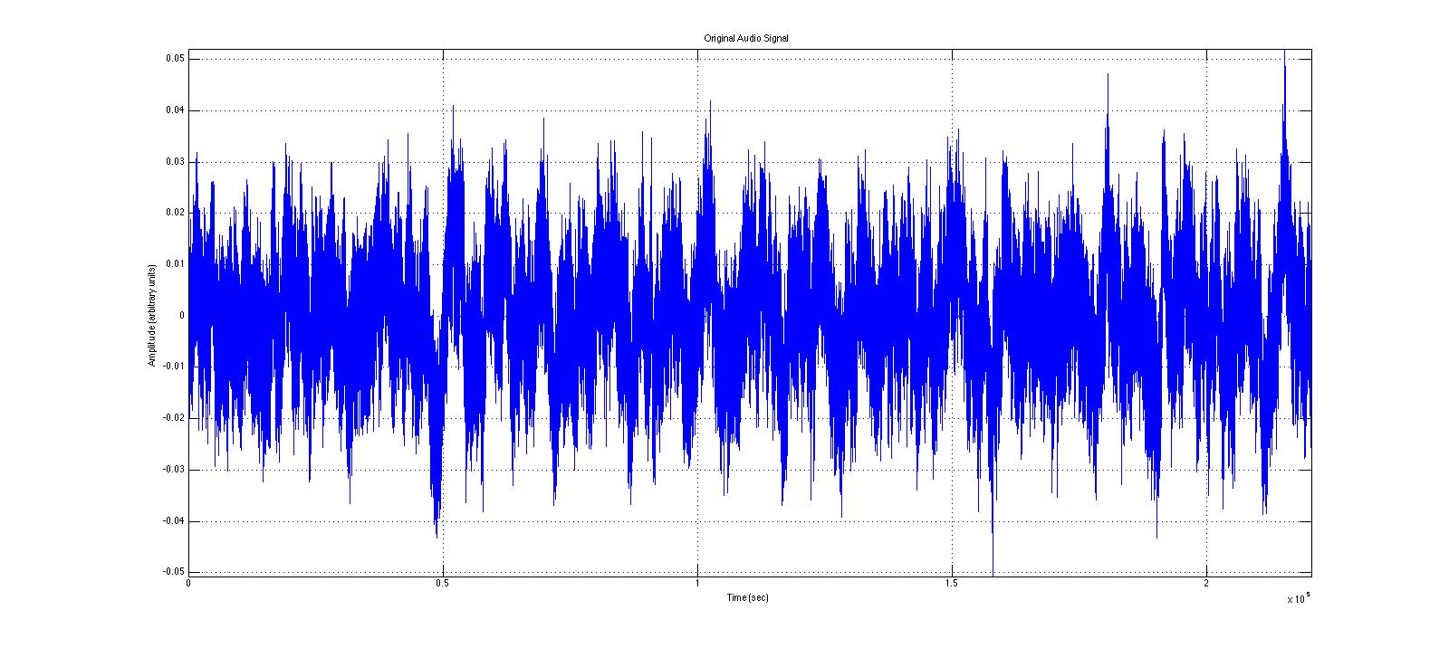
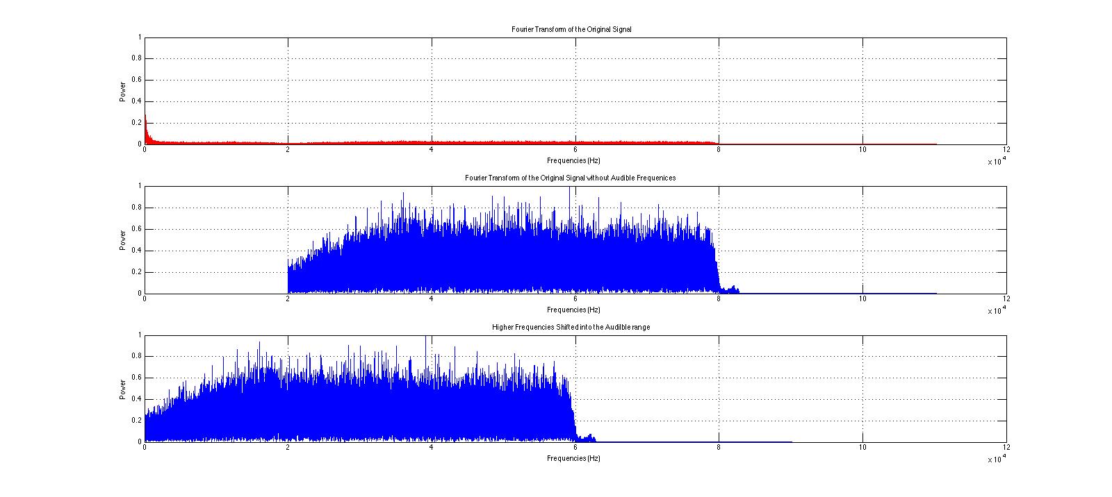
The program has three main sections. First, matrices are created to store the relevant results and initial parameters of the system. Then the input EMG code is chopped into bins .1 seconds in length and each bin progresses through the rest of the code sequentially and independently. From this, the chopped data is passed through a Fourier transform, and the major sources of noise are excised. The excised noise sources are as follows: <20 Hz noise originating primarily from movement artifacts and low frequency pressure waves and 60 Hz noise stemming from most electrical appliances and lights.

The second section solves for the spike amplitudes in each bin. Using the findpeaks command, the locations and magnitudes of each of the spikes are solved for using nested if/else and while loops. The locations of each of the peaks are passed into the third section, while the peak amplitudes are saved as one of the output parameters.

The third section solves for the spike duration and splits the signal into each regime. To do so, a series of nested if/else and while loops are set to proceed from each spike and the beginning of the bin. First, the spike durations are calculated using the locations of the peak amplitudes from the previous section of code. After the spike durations are found, the code cycles back and calculates the regimes where the arm is considered to be either holding  or going to a rest state. Any excess time within the bin created as a result of conditions to maintain code stability is then characterized as a hold state, which will allow the physical Neuroprosthetic arm to catch up to the computation in the physical system. The final output durations are then tagged according to which regime they belong into and the results are output in a cycle durations matrix for each bin.

A fourth section, which is only utilized if no spikes are detected in the current bin, goes through the same procedure of finding the hold and rest regime durations for the inactive bins.

In the code graphs of the original signal, comparisons of the rectified and original signals for each bin and the total program are created to allow the experimenter to have a visual verification of the efficacy of the code.

Results:

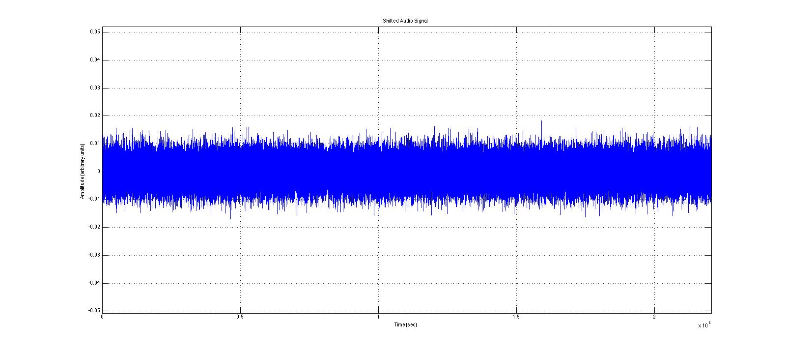
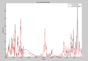
As discussed previously, the code was both successful and stable. Following the Fourier noise rectification, the signal was clearer and more legible than the original signal, and the data was still maintained. The peak amplitude outputs are accurate, and are positioned in the output matrices identically to their corresponding spike duration for easy identification and analysis. Similarly, the code successfully found the regime durations in each bin, with hold, contracting and resting states all distinguishable and present in the appropriate locations and placed sequentially.

Analysis of the output signal figure will shows the noise reduction caused as a result of the Fourier noise analysis, and the table, showing the output cycle duration matrix, shows how cycle durations were successfully found. To see larger images, please see either the google drive folder associated with this project, or click on the images themselves.

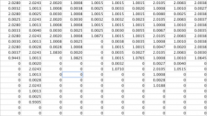
Conclusion and Future Experiments

I am satisfied with this initial foray into Neuroprosthetic data mining. The data outputs were accurate and returned the information that I sought to solve. Furthermore, the architecture of this code is easily transferable to other formats and coding languages, and can be modified to solve for other experimental parameters dependent on the needs of the other experiments.

Although in and of itself, this experiment is extremely successful, and wide number of individual parameters can be calculated by altering the analysis code slightly, the architecture itself may prove unsatisfactory in later experiments. The reason for this is that this code currently only processes data stemming from a single data input. However, there are a number of models for nerve activity that are reliant upon populations and pre-contraction initial conditions (Churchland, 2012), which are significantly more complicated and cannot be solved for using the current architecture. However, I believe that it is not necessary to use that kind of population level model, in which case this architecture is sufficient for later work.

Further modifications to this code will be to change the parameters that the code solves for, as well as transferring the code Arduino such that it can be installed directly into the robot arm. Furthermore, there is a significant amount of information lost through data processing in the name of preventing crashes, which is an inefficiency that I intend to remove in the future. The code developed for this project will serve as an initial, rudimentary data mining code which can be used in a number of different ways elsewhere in my future projects and investigations into neuroprosthetics.

Relevant Files can be found through the link below with headers:

1: EMG_Data_Analysis_427.m

2: SampleEMG1.mat

3: SampleEMG2.mat

4: SampleEMG3.mat

https://drive.google.com/drive/#folders/0B0K4JjJfDy1ffkR4eEZaMzlxb0xvTjRjWDBIUm9iVzZuRmVyeG1aM0RhWHMxcVB6RXZDUFk

References:

1: De Luca, C. Gilmore, D. Kuznetsov, M. Roy, S. Filtering the surface EMG signal: Movement artifact and Baseline noise contamination. Journal of Biomechanics (January 5, 2010) 1573-1579

2: Richards, C. Biewener, A. Modulation of in vivo power output during swimming in the African clawed frog. Journal of Experimental Biology 210 (2007) 3147-3159

3: Lichtwark, G. Wilson, A. A modified Hill muscle model that predicts muscle power output and efficiency during sinusoidal length changes. Journal of Experimental Biology 208 (2005) 2831-2843

4: Computational Physics by Nicholas J. Giordano and Hisao Nakanishi

5: Churchland, M. et. al. Neural population dynamics during reaching Nature (2012) 51-56

Introduction

As a fairly precise branch of physics, as well as one of the oldest, there are many problems in celestial mechanics for which an analytical solution is well known. Still, some problems exist for which an analytical solution is either very difficult or impossible to obtain. For the former, a computational analysis serves to verify analytical theory; for the latter, simulation may be the best way of understanding a problem other than with direct observation. The goal of this project is to examine two celestial mechanics problems with a computational model: the precession of the perihelion of Mercury and Kirkwood Gaps.

Precession of Perihelion

For centuries astronomies had a prediction of Mercury’s orbit from Kepler’s laws which measurably differed from observational values. What astronomers found was that Mercury mostly obeyed Newton’s inverse square law for its motion, but deviated because the orientation of the orbit’s axes was rotating over time. This is referred to as the precession of the perihelion, because the perihelion (the point in the orbit at which Mercury is closest to the Sun) lies along the semimajor axes. The source of the deviation from theory was a mystery until Albert Einstein released his paper on general relativity in 1915, in which he claimed his new theory explained the precession of the perihelion of Mercury due to the relativistic gravitational effects from the other planets (particularly Jupiter). Einstein’s adjustment to the inverse square force law is as follows:

The value for alpha shown above is the value calculated from general relativity; for this simulation, a much larger value of alpha is used so that the simulation doesn’t have to run as long to show precession. The value used in the main code of this program is .0008.

We then use the force law to calculate the velocity and position of Mercury. The derivation for the position and velocity with respect to x is as follows:

The derivation is virtually identical with respect to y. We then use these differential equations to create a computational algorithm; I chose to use the Runge-Kutta method because I felt that updating the values within the orbit computation loop would lead to a more accurate simulation.

A representative graph is also included to show how the orbit changes over time.

Now that we have a code for the movement of Mercury, the next step is to find where the perihelions of each orbit lie. I did so by first conceptualizing what happens at the perihelions. Because the perihelions are the most rounded parts of Mercury’s orbit, the change in the distance from the Sun will be very small or slightly negative as Mercury moves closer to the Sun. Using this knowledge, I then find the position at these points and convert it to an angle. Angle is then graphed against time to show how the perihelion precesses over time.

The goal of this graph is to find the fit slope of our angles so as to compare our computed precession rate to the analytical precession rate per unit alpha, 1.1 * 10^4 degrees per year per unit alpha. Using this value, we should be able to multiply it by the value of alpha predicted from general relativity to find a precession rate of about 1.2 * 10^4 degrees per year, or 43 arcseconds per century.

Continuing the program, I ran the precession simulation for values of alpha from .0001 to .004. I then created arrays to hold these alphas and their corresponding precession rates per alpha and plotted both with a fit line. The slope of this graph multiplied by alpha from general relativity is compared to the analytical values.

The slope calculated from the angle vs. time graph was 8.4516 with an r value of .749. Therefore the precession rate per alpha here, calculated by slope/alpha, is 1.067*10^4 degrees/year/unit alpha, which compared to the analytical value is a relative error of 2.9%. This precession rate per alpha is then calculated again in the slope of the second graph, which comes out to 1.1139*10^4 degrees/year/unit alpha, a relative error of 1.9%. Multiplying by Einstein’s alpha, we find a precession rate of 1.2253*10^-4 degrees/year or 44.11 arcseconds/century, with relative errors of 2.1% and 2.6% respectively.

Kirkwood Gaps

When astronomer Daniel Kirkwood plotted the number of known asteroids against their orbital radii, he found significant “gaps” of asteroids- orbital radii at which few or no asteroids were found to exist. Eventually he discovered that these orbital radii were in resonance with Jupiter, the largest planet and, as seen by the precession of the perihelion of Mercury, therefore the most likely to perturb the orbits of other objects in the solar system. This resonance is a ratio of the orbital periods for two objects rotating around the same central body of mass, and is related to the orbital radii of the object.  So in this example this project, the orbital period of an asteroid located at the 2/1 resonance point with Jupiter will be one half that of Jupiter’s, so it will complete two orbits for every one Jupiter completes. The relation between orbital period and orbital radii is given by Kepler’s Third Law:

where P is orbital period and a is orbital radius; this proportion holds for all objects orbiting the Sun. Knowing that Jupiter’s orbital radius is 5.2 AU, we can calculate the position of asteroids at resonance points by this ratio; i.e. at the 2/1 resonance, the orbital radius is 3.27 AU, 2.5 AU at the 3/1 point, and so on. We can also use the calculated radius to find the initial velocity by the equation for orbital speed:

The reason why Jupiter perturbs the asteroids so much at these radii is due to resonance- because the object in resonance is closest to Jupiter at the same several points in its orbit (for example, twice in the orbit of the 2/1 resonance), the perturbations from Jupiter will be largest only here and cause highly erratic orbits over time. The same phenomenon doesn’t happen at other radii because Jupiter’s perturbations occur at random points on the asteroid’s orbit and altogether cancel each other out over time.

My code begins with the 3-body system as described on page 115 of Giordano and Nakanishi using the Euler-Cromer method. First I tested my code to demonstrate it worked without adding any asteroids:

Then I added asteroids at and around the 2/1 resonance point. Normally when adding more bodies to such a system, the new bodies interact with and change the orbits of the original objects, but because the mass of the asteroids is negligible as compared to all 3 objects already in the system (the Sun, Earth, and Jupiter), this effect can be ignored. The highly erratic 2/1 resonance is shown in blue:

The other two asteroids demonstrate how little Jupiter perturbs their orbits. I then added asteroids at the 3/1, 7/3, and 5/2 resonance points, but found a very different effect:

I originally thought that this was an error in the simulation, most likely caused by too many objects in the system, but I am now confident this is an accurate approximation of the involved physics; the explanation is in the following section.

Conclusion

Because the precession rate of Mercury has already been found analytically, it hardly comes as a surprise that the computational solution closely matches both theory and observation. The small relative errors compared to the analytical values shows the program is successful. While figuring out how to find the perihelion as it rotates was difficult, the rest of the program is straightforward because it follows from the known force equations. The program also demonstrates how known physical values can be altered to make computation easier, such as using a much larger alpha than in reality so as to speed up the calculation. While it might be more physically realistic to calculate the precession rate using a system with more massive bodies, at least including the largest perturber Jupiter, the calculated values are good enough to conclude the current simulation is sufficient in verisimilitude.

The program for the Kirkwood Gaps demonstrates how one very particular physical property, resonance, can have a very large effect when massive bodies are concerned. The first asteroid graph demonstrates this quite effectively, as the asteroid found in the 2/1 gap is perturbed much more than the outermost asteroid which is significantly closer to Jupiter. The graph of the other resonance points demonstrates exactly why it is that the Kirkwood gaps exist: eventually the perturbations from Jupiter become so large that the orbiting object is ejected entirely. The asteroid at the 2/1 resonance point isn’t ejected because it has the lowest frequency of interaction with Jupiter. At the other resonance points, Jupiter perturbs its orbit enough to eject it, because of the higher rate of encounter- the asteroid at the 3/1 resonance point is effected by Jupiter one more time than the 2/1 asteroid per orbit, a difference which has significant consequences over time. This program serves as a successful example of how a computational simulation can lead to greater understanding of the underlying physics even when an exact answer isn’t possible or even necessary. It is also worth noting that a phenomenon similar to Kirkwood gaps occurs with the rings of planets; for a real-life example, the rings of Saturn have gaps in them because the gaps are in resonance with one of Saturn’s moons.

Code:

https://drivenotepad.appspot.com/app?state=%7B%22ids%22:%5B%220B0gZLI_X8KZXWkxEbHVEVHlLbjQ%22%5D,%22action%22:%22open%22,%22userId%22:%22116986450796621489073%22%7D

https://drivenotepad.appspot.com/app?state=%7B%22ids%22:%5B%220B0gZLI_X8KZXSHNTaWlLQkhfZE0%22%5D,%22action%22:%22open%22,%22userId%22:%22116986450796621489073%22%7D

https://drivenotepad.appspot.com/app?state=%7B%22ids%22:%5B%220B0gZLI_X8KZXWlV3aDZFQThhaFk%22%5D,%22action%22:%22open%22,%22userId%22:%22116986450796621489073%22%7D

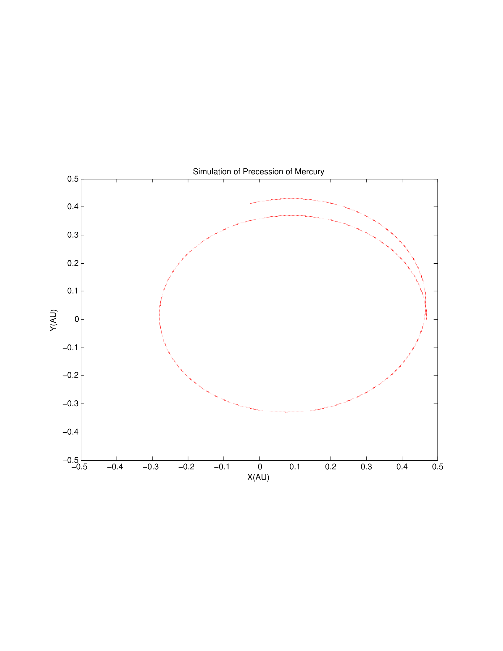
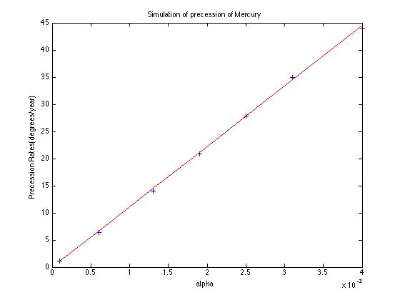
The precession of Mercury is caused by the gravitational effects of the other planets (Jupiter contributing the most) and the general relativistic effects of the Sun. In the first part of my project I set about achieving the value of the precession of Mercury using the Euler-Chromer method to simulate Mercury’s orbit and least-square linear fits of and precession rate vs. . I achieved a value of , with a percent error deviation of 10.39 from the true value, .

In the second part of my project, I let the eccentricity of the orbit of a Mercurian-sized body vary in its orbit in order to observe eccentricity’s effect on the precession rate. I determined that precession rate is inversely proportional to . The values of and eccentricity I used are included in a table attached to this post.

This past week I experimented with 3-body systems in order to determine the effect of Jupiter on Mercury’s precession. Using the Euler-Chromer method I was able to successfully model a Jupiter-Mercury-Sun system, but only when the Sun’s position and velocity were held at 0.

For the case in which the Sun was to be given an initial position and velocity, I input parameters that should have allowed the center of mass to remain constant, however the graphs showed the Sun escaping from the solar system. Unfortunately I’m not sure how this error occurred, however I am convinced that this model is necessary to determine Jupiter’s effect on Mercury’s precession, as I was unable to achieve the correct value with the model in which the Sun’s position and velocity were held constant.

Link to Code:
https://docs.google.com/a/vassar.edu/document/d/1DrX3F-mnJsyuq8FPltXRY8aCFyNxQvoUGUG_BoIpiBE/edit?usp=sharing

Link to Eccentricity Data:
https://docs.google.com/a/vassar.edu/spreadsheets/d/1YNlhVNkyhy-arqPQW5dAoME6pCHRKIlXpKaZ6bisG-s/edit?usp=sharing

Introduction

Our initial plans for this project were to model and guitar string, piano string, and drum head in MatLab, then compare data calculated to a real scenario, using the physical instruments and recording the sounds they create.  We were able to complete the guitar and piano strings, but were not able to advance to the drum head due to time constraints.  However, we did get a lot of good data from our experiments with the guitar and piano strings.

Guitar String

For this part of our project, we modeled a guitar’s B string in MatLab, and plucked the string at different points: once at the midpoint of the string, once 1/5 the string length from the bridge, and once 1/20 the string length from the bridge.  In the proceeding images, you can see the string oscillations, the force of the string on the guitar bridge with respect to time, and the Fourier Transform of these force graphs, which reveal the frequencies inside.

Modeled Guitar Data:

Frequencies of waveforms (Fourier Transform):

The force of the string on the bridge with respect to time is nearly identical to the sound wave that the string produces in the atmosphere, thus we were able to use that data to find the frequencies in our calculated string.  We also shifted the frequencies on the graph of the Fourier Transform for visual purposes (if not shifted, they would line up on top of each other and be difficult to distinguish).

Next, we recorded a guitar B string, identical to the one we modeled, and Fourier transformed those recordings to obtain the frequencies inside.

Frequencies of Physical Guitar String:

Here are the recorded guitar sound files.  Note as the pluck gets closer to the bridge, the tone of the guitar becomes harsher.  We will discuss this soon.

String Plucked at (1/2) distance:

String Plucked at (1/5) distance:

String plucked at (1/20) distance:

In our code for the modeled guitar string, the calculated waveform is played for the viewer, and as seen from the physical guitar, the tone of the sound gets harsher as the pluck gets closer to the bridge.  This harsher sound is the stronger presence of the overtones in the waveform as seen in our Fourier transforms.  As the pluck gets closer to the bridge, strength of the higher frequencies increases, which is why the sounds produced becomes much harsher.  This is what we expected and found with this part of the experiment.  Comparing our Fourier transform graphs, we see that the peaks at the higher frequencies increase with each pluck closer to the bridge.  We can also see that the closer the pluck is to the bridge, the lower the fundamental frequency becomes present in the produced sound.

However, there are some inconsistencies between the modeled and physical strings.  The modeled string did not contain and decaying properties, where the physical string did.  Also, the modeled string data was calculated using two dimensions when the physicals string would utilize all 3.   This important difference shows in the Fourier Transform of the modeled string.  When the modeled string is plucked at the halfway point, every other frequency (or peak) is eliminated from the Fourier transform; same as when plucked at 1/5, the fifth and tenth peak is eliminated.  In this modeled state, we are effectively killing these overtones by plucking where they would naturally occur on the string.  The decay properties of the physical string allow these “ghosted” frequencies to sound because the string can move freely rather than stay in a fixed 2-D dimension and fixed wave profile.  Another reason behind this, could be that the physical string is not of ideal form, meaning it is a series of coiled wires rather than a solid string.  This could have imperfections giving rise to these “ghosted” frequencies.

Another small discrepancy in our data is that the fundamental frequency of the physical string plucked at the halfway point is lower than when plucked at the other distances.  We don’t see this in our modeled system because the amplitude of the pluck was held constant for each pluck (giving us the results we expect).  On the physical string, the string is able to bend more at the middle than closer to the bridge.  Thus to get an equal volume pluck, we must do a harder pluck in the middle than closer to the bridge.  If we kept the amplitude of the plucks for the physical guitar the same, we would expected the power of the individual frequencies to closer match the modeled ones.

Piano String

For this part of our project, we modeled a piano’s middle C string in MatLab, and struck the string with different forces: Once softly, and once more powerfully.  In the proceeding images, you can see the string oscillations, the force of the string on the piano bridge with respect to time, and the Fourier Transform of these force graphs, which reveal the frequencies inside, all for two different hit intensities.

The model included a hammer with mass and an original velocity (which changes between the two trials) as well as a felt on the hammer which behaves as a spring. Here the compression of the felt is dependent on the position of the hammer and the string section where the hammer strikes, and which affects the positions of the freely moving hammer and string based on its compression. When the compression changes signs, we know that the hammer has left the string and we automatically give the string no outside force.

Modeled Piano Data and Frequencies

The force of the string on the bridge with respect to time is nearly identical to the sound wave that the string produces in the atmosphere, thus we were able to use that data to find the frequencies in our calculated string.

Next, we recorded a piano C string, identical to the one we modeled, and Fourier transformed those recordings to obtain the frequencies inside.

Frequencies of Real Piano String

Here are the recorded piano sound files.  Note when the strike is harder, the tone of the guitar becomes harsher.  We will discuss this soon.

Hard String Hit:

Soft String Hit:

In our code for the modeled piano string, as the strike gets harder, strength of the higher frequencies increases, which is why the sounds produced becomes much harsher.  This is what we expected and found with our simulations.  A similar trend was also found in the Fourier transformed recorded sound files.

However, there are some inconsistencies between the modeled and physical strings. One such difference was the lower fundamental frequency than the second overtone in the recordings, as compared to our model. This could be due to the amplifying qualities of the piano box. The modeled string did not contain and decaying properties, where the physical string did.  Also, the modeled string data was calculated using two dimensions when the physicals string would utilize all 3.  The model we simulated made assumptions about the spring like qualities of the felt, the width of the hammer, as well as the strike intensity, which we couldn’t make equivalent to the recorded strikes. This created some strange differences, including a strangely sharp hammer hit (not as soft as one might expect from a spring, as well as differing from the textbook’s predicted hammer behavior). We brainstormed what may be it’s cause (the hammer velocity, the original felt thickness, the hammer’s strike position) but couldn’t find a solution.

Conclusion

In conclusion our results were what we expected with some degree of uncertainty. String plucks closer to the bridge and harder string strikes produce more overtone notes relative to the fundamental frequency. If we had more time/if this project were to continue further, we would explore the addition of a damping coefficient in our modeled experiments and compare with physical strings, investigating the discrepancies mentioned earlier.  We would also begin to explore the drum head dynamics, experimenting with two 3-D membranes, connected through a closed hoop, similar to the structure of an actual drum.

The following link is to a google drive containing all of our code and sound files.

https://drive.google.com/folderview?id=0ByhnW_B9B6q9flE5bWtTal9Yd19ZYzhrOGpUbjctMUhIM3FMRGxvMDVMZkF3NUJSbFJ1MEU&usp=sharing

Please note, if you are planning to run the code that involves the recordings of the instruments, YOU MUST CHANGE THE DIRECTORY IN WHICH THE CODE CALLS THE SOUND FILE.  Each space in the code is noted where this part should be edited.  This needs to be done as the naming of folders and drives varies from computer to computer.  Not only must the correct location of the file be used, but the sound files must be saved in the same location as the MatLab code or it will not run.  Also the correct sound file must be called in each spot, or the sampling will be off/ the code will not run properly.