Tag Archives: computational

Simulation of a Squash Ball

squashball3

The data generated in my project consisted of position data for the path of a squash ball in motion in the spatial context of a squash court. Additional important generated data included the velocity of the ball (in 3-dimensions) at any given time. Euler’s method was a relatively practical numerical method, as it made calculating the position at each step of dt (which was imperative in the animation aspect of the project) a simple matter of using the position and velocity information from the previous time step.

Some difficulty arose in attempting to achieve a smooth animation, due partly to computational time. Ultimately the solution for animating the path of the squash balls necessitated creating matrices for the position of the ball in each dimension in Cartesian coordinates. After this, the comet3 function was used to animate the plot, as it the head of the comet nicely approximated the shape of a ball, and the tail was very useful in showing the entire path of the ball from its initial position.

In the end, my goals for the project had to be altered slightly, as attaining the user-friendly inputs that I had wanted proved to be a complicated task. I had initially hoped that the finished product would allow for a user to input some initial velocity using the arrow keys. Ideally the user would hold down some combination of the arrow keys for some amount of time, and then press the spacebar to initialize the loop and set the ball in motion. Based on the amount of time each direction arrow had been pressed, the ball would be imparted with a corresponding initial velocity. However, unfortunately Matlab’s capabilities to not allow for the reading of key presses without the use of user-generated GUI’s. Given that my understanding remains relatively basic, I had to scrap my dreams of user-interaction with the model.

Though the ultimate goal of my script was an educational experience for the user, writing the script was a learning experience in itself. I had previously modeled some colliding pendulums in Matlab, and I drew on this code in scripting the ball-to-wall collisions, and subsequently the resultant velocities of the ball was an easy task. In the early draft of my code I encountered some problems, as certain initial velocities seemed to result in the ball getting stuck inside the walls – an obviously undesirable result due to its physical improbability. Having encountered a similar issue in my colliding pendulums code, I knew that the problem had something to do with the script not checking on the position of the ball often enough, due to the time step, ‘dt’, being too large. While this was part of the problem, the larger source of the issue was the fact that, once beyond the wall, the ball’s velocity was rapidly decreasing, as the script believed that it was continuously colliding with the wall. In the end the fix was relatively simple: if the ball passes beyond the wall, reset the balls position so that it is at the wall again. Though simplistic, this is a powerful idea in the context of computational methods. If having a variable reach a target value is desirable for your simulation or simplifies the problem, just check that the variable comes within a reasonable range and set it to the target value.

squashbirdseye

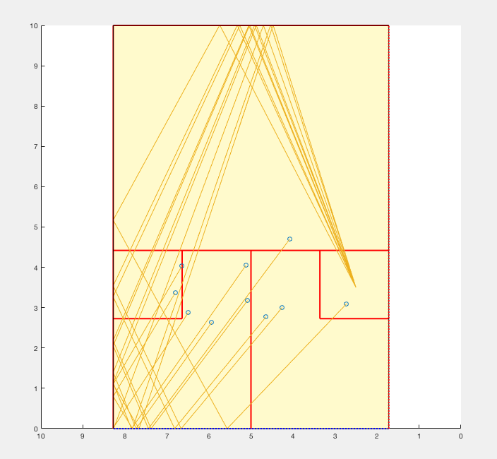
I was surprised to note how relatively close to the front and right wall many of the balls ended up. This was most likely due to the fact that my expectations came from having played squash. When returning the serve, the goal is to hit the ball back before it bounces twice, therefore if you have watched to ball until it stops rolling (as the script does), you have long since lost the point. It was interesting to confirm that the majority of serves bounce twice within the confines of the larger box in the back left of the court (makes up about a quarter of the floor) which verified my own experience that almost all serves are returned from the back left of the court. Though these results seem quite inconsequential, the objective of the script is an educational experience, so these observations can be read as positive outcomes.

The goal of my script was entirely focused on user experience. Consequently, the product of the script was not heavy on calculated results. The main idea was for users to be able to gain an intuition for the flight path of a squash serve without ever having played, or even seen the sport being played before. On the other hand, it may have been interesting to take the project in a more numerical-result-driven direction. For instance, a comparison of the initial angle of the ball with the final angle would have made for an interesting discussion. Having run through the script a number of times, and therefore seen at least a hundred individual ball paths fully plotted, a distinction between the serves that struck the side-wall before the back-wall, and those that did the opposite definitely emerged. Quantifying this difference could potentially be illuminating. Another question that might be considered concerns the balls that hit the side-wall and back-wall simultaneously. How would these corner cases (pun intended) show up in the data? If I were to modify the script to accomplish this, the most important change would be to increase the number of iterations from ten into the hundreds or even thousands. This would almost certainly necessitate abandoning the full animation of the flight path, and focusing instead on the location of the ball’s second bounce on the floor (when, according to the rules of squash, the point has ended).

If I were to instead expand my project to expand the user’s experience and fully embrace the educational aspect of the project, I would certainly want to solve the problem of more interactive user input. Allowing the user to control the velocity would allow them to develop a feel for the serve without ever having stepped on a court, whereas the project in its current state relegates the user to the role of an observer, rather than an active participant. Ideally the project could be taken beyond the confines of a serve, and allow the user to control a player that plays out a full point, perhaps against a computer-controlled player. This would potentially require quite complex user input capabilities (for position of the player and velocity and direction of each hit) and would also necessitate a method of plotting that was instantaneous. A more simplistic full-point simulation could also be created by creating additional collision areas that represent swinging rackets at various locations the court, so that a ball that happened to reach that position would be imparted with some new velocity and direction.

Sources:

<http://www.worldsquash.org/ws/resources/court-construction>

<http://www.worldsquash.org/ws/resources/rackets-balls/racket-ball-specifications>

Share

Molecular Dynamics Project Conclusions

Molecular Dynamics Project Summary

Sushant Mahat and Mohammed Abdelaziz

Over the last few weeks, we have been working on a computational project on molecular dynamics. This post below summarizes the details of this project, and the overall goals we achieved.


Initial Goals and Motivations:

We wanted to do an experiment in molecular dynamics as it connects to several things we have studied in our previous physics classes. We used our knowledge on Newton’s second law which we learned in classical mechanics; we used Boltzmann’s distribution and the concepts of temperature from thermodynamics and statistical mechanics; and we used the Lennard-Jones potential which has its root in quantum mechanics. All these features made simulating  molecular dynamics an attractive, challenging, and a very educational project.

We had several goals when we started this project. We wanted to be able to simulate a 2-D gas system, and be able to study several of its properties like temperature, energies, speed distributions, and visualization at equilibrium. We then wanted to build up on this system to make it into a 3-D system. We were also thinking about making it possible to increase the temperature of the system and observe how long it takes to come back to equilibrium. This was supposed to be a simulation of periodic heating of gas particles with a laser beam.


Goals We Completed

Due to time constraints, we were unable to fulfill some of our initial goals. However, we were able to finish most of the goals. The goals we met for this project include:

  1. Simulating the motion of a dilute sample of gaseous Argon atoms in two dimensions.
  2. Calculating the mean velocities of each atom and plotting their speed distribution in each simulation.
  3. Determining the temperature of the sample based on initial and equilibrium speeds of each atom, which required a determination of the kinetic energies of all atoms at each time step.
  4. Comparing the calculated speed distribution with the Maxwell-Boltzmann speed distribution curve.
  5. Completing the simulation and the above calculations in three dimensions.
  6. Introduced possibility to simulate temperature change in the system.


Methods

Section 9.1 of Giordano and Nakanishi’s Computational Physics was our primary reference for this project. We used MATLAB for the simulations, dividing our code into several functions (subroutines) instead of using one script. The codes and their purposes are outlined below.


TheInitiator.m

This function initializes an evenly spaced grid in 3-D space (2-D in the old version of the program). This grid serves as the basis for the location of each atom, because we want the atoms to start at roughly the same location for each simulation. Two further steps are taken to make sure the simulations are not fully deterministic: each atom was displaced slightly from a point on this evenly spaced grid, and it was given a random velocity (within some limits) in each dimension. This function also allows an option to have different limits of the initial random velocity which can produce an effect similar to starting with gas particles with different temperature.


TheEnforcer.m

This function calculates the force on each atom due to every other atom, based on the Lennard-Jones potential, which is ineffective at large distances, attractive at moderate distances, and repulsive at very short distances. This calculation takes exponentially longer for additional particles, because each particle interacts with each other particle.


TheUpdater.m

This function uses the forces from the previous function and each particle’s positions to calculate each particle’s position and velocity at the next time step. It feeds these positions back into TheEnforcer.m and iterates until the positions and velocities of each particle for each time step are calculated. This function also enforces the periodic boundary conditions (that a particle leaving one side of the “box” comes back through the other side, with its velocity unaffected). Particles that are closer to each other through these boundary conditions than they appear must interact as though they were at this close distance. To clarify this, consider a one-dimensional system, ranging from x=0 to x=10. Two particles at x=1 and x=9 should interact as if they are 2 units apart, not 8 units apart. Implementing this system properly was one of the most difficult tasks we faced.


SpeedDist.m

This function takes in each velocity component of each particle at each time step, and first calculates a speed for each particle at each time step. It plots three speed distribution curves by averaging each particle’s speed over each third of the runtime, placing these speeds into bins, and plotting a histogram that is visualized as a curve. The function is configurable to plot any integer D speed distribution curves by averaging each particle’s speed over each 1/D of the runtime instead, but D = 3 effectively showed that the system had reached equilibrium (signified by when two successive speed distribution curves are fairly similar).

This function also plots the kinetic, potential, and total energy averaged for all particles at each time step in the simulation. The kinetic energy was needed to calculate temperature, since the product of Boltzmann’s constant and the system’s temperature is equal to the average kinetic energy of all particles in the system.


MainBody.m

This script simply initializes the spatial dimensions of the system and how many atoms will be simulated. This is the code that is directly run by the user to visualize the simulation and look at the speed distributions and energies.

All of these MATLAB files can be found in this Google Drive folder.


Results

We succeeded in producing visualizations of the Argon atoms in two and three dimensions. Even with 100 atoms, the script does not take more than thirty seconds to run, so more particles could feasibly be simulated. Additionally, our speed distributions matched up relatively well with the actual Maxwell-Boltzmann distributions in terms of horizontal location (this shows that our determination of temperature was accurate, since this is what affects the horizontal position of the peak (most common particle speed). However, our generated speed distributions were more narrow than the Maxwell-Boltzmann distribution. It is possible that they could be widened by decreasing the density of the atoms (simulating fewer particles or making the dimensions of the “box” bigger). It is also possible that increasing the maximum initial velocity would increase the width of the speed distribution, since it would give each particle a wider range of initial velocities to have.

We were mostly satisfied with our energy plots; they showed a fairly constant total energy, which we expect (it is not completely constant because the total energy is calculated from averages of kinetic and potential energy of all particles). Kinetic and potential energies became steady as the system reached equilibrium, which takes longer for lower gas densities.

One example of a speed distribution plot (click for full-size):

speedDistImage

One example of an energy plot (click for full-size):

energies


Conclusion and Future Potential

Based on the Boltzmann’s distribution plots of our data, we are fairly confident that our simulation is useful at approximating systems of gas molecules. The fact that the total energy of the system remains around a fixed value is also promising. However, the fluctuations in the total energy when the particles start interacting is still not ideal.

One limitation of our problem would be that the system destabilizes when the initial density of our gas molecules are very high. This is a direct result of the steep increase in the Lennard-Jones potential at low distances between particles.

We want our readers to see this code as a work in progress rather than a complete program. The program still has a lot of unrealized potential. For example, the energy graph produced by the simulation for cases with different initial velocity limits could potentially be used to calculate time taken by a system with gases of different temperature to equilibrate. Similarly, with some changes to the initiator and the enforcer function, the program could also be used to simulate a collection of different gases as opposed to a single type of gas molecule. Although we were unable to simulate it, increasing the density and lowering the initial velocity should also make it possible for future users to simulate materials in solid and liquid phases. Since the program already has method to change temperature built into it, some changes could be made to make these temperature changes periodic. This could potentially be used to simulate a laser beam heating the gas particles.

Overall, we are very satisfied with the progress we were able to make throughout the semester. Apart from learning a great deal about different physical concepts, we also developed a deeper appreciation and knowledge of computational approaches towards studying physical systems. We also think that we have developed  a fair understanding of the limitations and the potential of the computational tools available to us, and we are confident that this project has prepared us for many more simulations that we are likely to encounter in our careers as physicists.         

Share