Tag Archives: Conclusion

Audio Signal Processing – Conclusion

Goal:

Our final program takes an acoustic wave signal, strips out all audible frequencies using a Fourier transform, then shifts a range of the ultrasound frequencies into the audible range in order to qualitatively investigate the properties of the audio signal. Our initial goal was to record our own ultrasound frequency signals for analysis, but we were not able to procure a microphone sensitive enough to record ultrasound. Instead we choose an online video claiming to repel rodents by emitting an audio wave with ultrasound frequencies that effect rats (found here: https://www.youtube.com/watch?v=l5x1Bb9UTT0). On first inspection, the signal seemed to only play what resembled white noise, but we needed an accurate representation of the frequencies present in the audio file before making any more assessments. We hypothesized that the video did not contain ultrasound frequencies capable of repelling rodents.

Investigation:

Using the frequency analysis methods we implemented earlier in our project we found that the video actually contained frequencies above 20 kHz. But we were still skeptical because these higher frequencies were about 80% less powerful than the frequencies present in the audible range. This may have been a tactic used to trick the user in believing that high frequency sounds were playing. We wanted to examine what the high frequencies sounded like so we took a 5 second clip from the audio file to scrutinize.

(Please find the 5 second clip here: https://drive.google.com/file/d/0B4quZV7NVNf7YU16blYwcUxXYXc/view?usp=sharing)

We started by removing any audible frequencies from the clip then shifted the ultrasound range into the audible. The resulting sound was again white noise, but at a lower volume.

(No audible frequencies: https://drive.google.com/file/d/0B4quZV7NVNf7clBFTlJIT1I5bzQ/view?usp=sharing , Shifted signal: https://drive.google.com/file/d/0B4quZV7NVNf7amhqVkZ6NjBtUXc/view?usp=sharing)

A qualitative analysis of this new wave does not lead us to believe this video would repel anything. White noise is not an abrasive sound unless played at extremely high volumes, but anything played at a high enough volume can be found abrasive. White noise is generally considered to be the exact opposite and there are white noise generators that are sold on the premise that they are calming and relaxing, and are used to help people focus or sleep. The video we analyzed is not exactly what we would expect in a rat repellent, it seems like this video aims to be more of an aid that would assist in rat mediation.

(code here: https://drive.google.com/file/d/0B4quZV7NVNf7cldUbG5WQUFWTXM/view?usp=sharing)

Virgin Wave

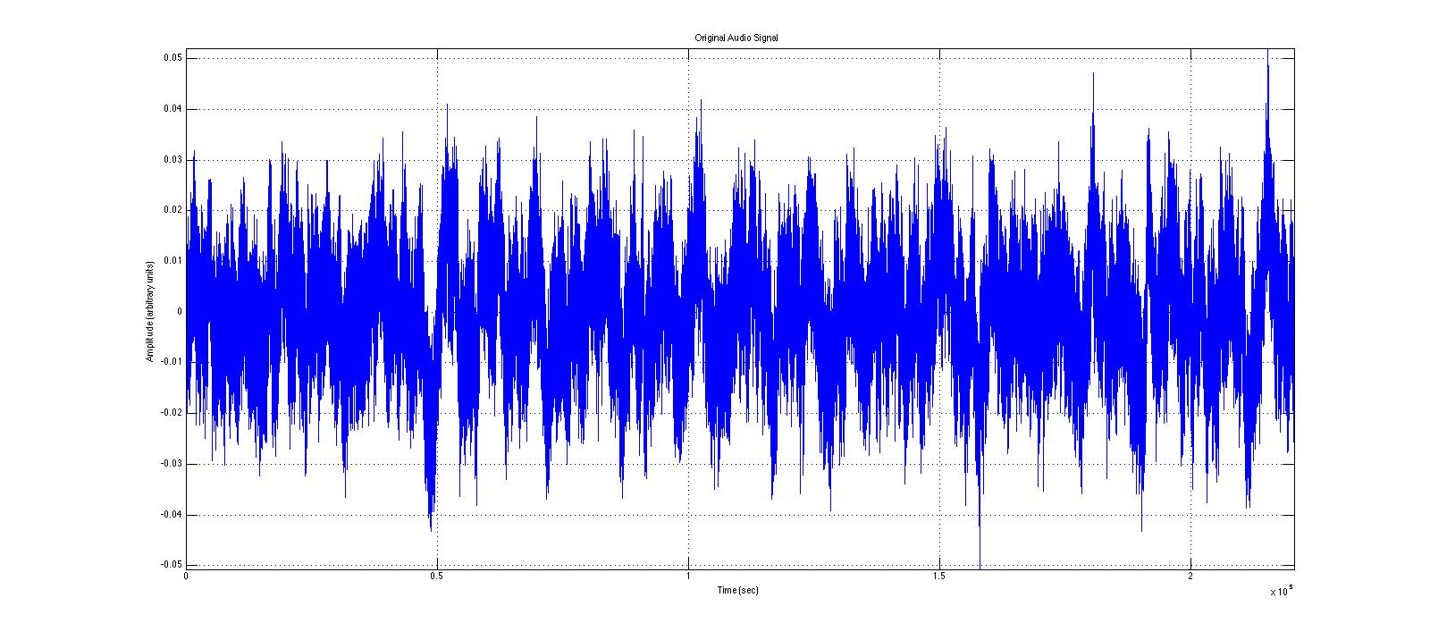
Here is the clip from the original 5 minute video. Notice the amplitude of this signal.

Analysis of Frequencies

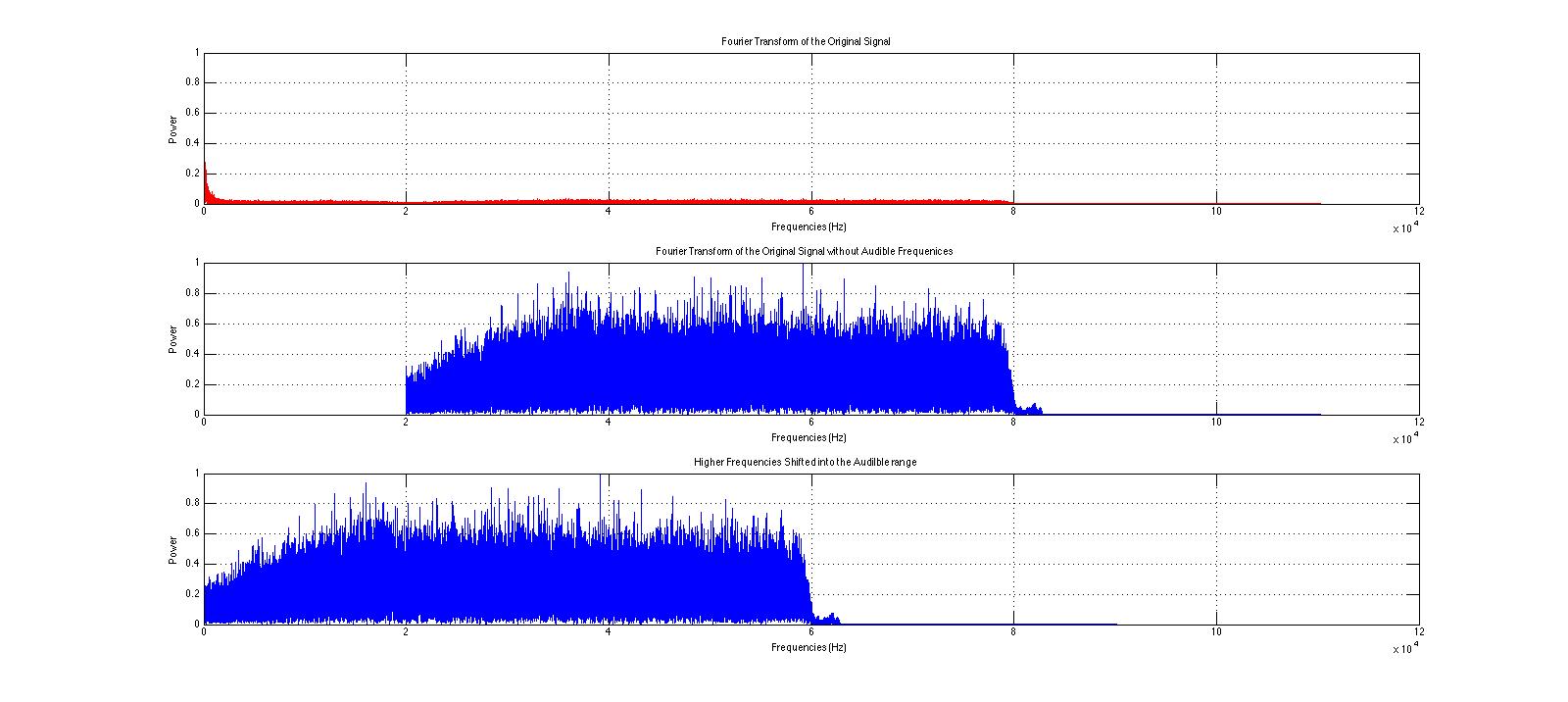
Here are the various operations we performed on the Fourier transform of the clip.

Audio Signal Without Audible Frequencies

No audible frequencies are present in this new signal. Please note the difference in amplitude in this signal from the original signal.

Shifted Signal

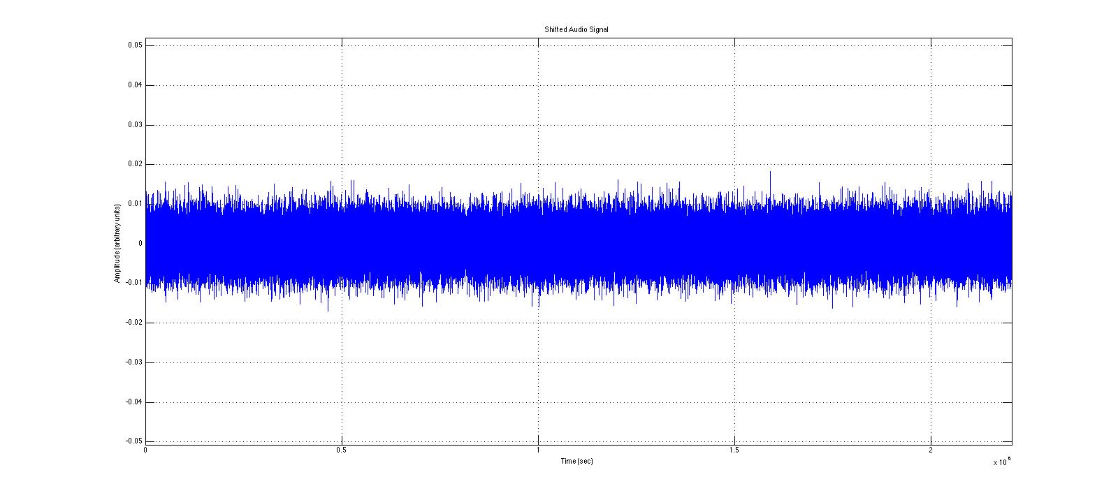
The new, shifted audio signal.

We then decided to make a code to demonstrate what a real rodent repellent signal might sounds like. We start by assuming that sounds that are irritating to humans are also irritating to rodents. A sound that is often considered to be annoying to us is a pair of high frequency sinusoidal waves that are similar in frequency but not identical. This is a very dissonant sound, and even at low volumes can grab the negative attention of someone around you (which can happen if you accidentally sound them in a public space while coding a rat repellent). So we also built a code that generates what we consider to be an abrasive sound, but is well above the audible range so we cannot hear it. We decided on the frequencies of a distressed rat baby (http://www.ratbehavior.org/rathearing.htm). Unfortunately, Matlab’s audiowrite function was not able to save this as a .mp3 file, so please download the code play and use the sound command found to play it on your machine.

(code here: https://drive.google.com/file/d/0B4quZV7NVNf7OW1kQld5QW1KVkk/view?usp=sharing)

 Future Work:

If we were to continue to research methods and applications frequency shifting we would write a code that transposes frequencies. Transposition maintains the harmonic ratios of the frequencies present in the wavefunction by multiplying them by a constant instead of linearly shifting them. Changing the sampling frequency at playback also maintain these ratios but in doing so, distorts the audio signal by stretching or compressing the wavefunction. Out next code would have been to transpose frequencies without changing the length of audio sample. We would also like to to detect our own ultrasound frequencies with an ultrasound microphone for qualitative analysis.

Share

Molecular Dynamics Project Conclusions

Molecular Dynamics Project Summary

Sushant Mahat and Mohammed Abdelaziz

Over the last few weeks, we have been working on a computational project on molecular dynamics. This post below summarizes the details of this project, and the overall goals we achieved.


Initial Goals and Motivations:

We wanted to do an experiment in molecular dynamics as it connects to several things we have studied in our previous physics classes. We used our knowledge on Newton’s second law which we learned in classical mechanics; we used Boltzmann’s distribution and the concepts of temperature from thermodynamics and statistical mechanics; and we used the Lennard-Jones potential which has its root in quantum mechanics. All these features made simulating  molecular dynamics an attractive, challenging, and a very educational project.

We had several goals when we started this project. We wanted to be able to simulate a 2-D gas system, and be able to study several of its properties like temperature, energies, speed distributions, and visualization at equilibrium. We then wanted to build up on this system to make it into a 3-D system. We were also thinking about making it possible to increase the temperature of the system and observe how long it takes to come back to equilibrium. This was supposed to be a simulation of periodic heating of gas particles with a laser beam.


Goals We Completed

Due to time constraints, we were unable to fulfill some of our initial goals. However, we were able to finish most of the goals. The goals we met for this project include:

  1. Simulating the motion of a dilute sample of gaseous Argon atoms in two dimensions.
  2. Calculating the mean velocities of each atom and plotting their speed distribution in each simulation.
  3. Determining the temperature of the sample based on initial and equilibrium speeds of each atom, which required a determination of the kinetic energies of all atoms at each time step.
  4. Comparing the calculated speed distribution with the Maxwell-Boltzmann speed distribution curve.
  5. Completing the simulation and the above calculations in three dimensions.
  6. Introduced possibility to simulate temperature change in the system.


Methods

Section 9.1 of Giordano and Nakanishi’s Computational Physics was our primary reference for this project. We used MATLAB for the simulations, dividing our code into several functions (subroutines) instead of using one script. The codes and their purposes are outlined below.


TheInitiator.m

This function initializes an evenly spaced grid in 3-D space (2-D in the old version of the program). This grid serves as the basis for the location of each atom, because we want the atoms to start at roughly the same location for each simulation. Two further steps are taken to make sure the simulations are not fully deterministic: each atom was displaced slightly from a point on this evenly spaced grid, and it was given a random velocity (within some limits) in each dimension. This function also allows an option to have different limits of the initial random velocity which can produce an effect similar to starting with gas particles with different temperature.


TheEnforcer.m

This function calculates the force on each atom due to every other atom, based on the Lennard-Jones potential, which is ineffective at large distances, attractive at moderate distances, and repulsive at very short distances. This calculation takes exponentially longer for additional particles, because each particle interacts with each other particle.


TheUpdater.m

This function uses the forces from the previous function and each particle’s positions to calculate each particle’s position and velocity at the next time step. It feeds these positions back into TheEnforcer.m and iterates until the positions and velocities of each particle for each time step are calculated. This function also enforces the periodic boundary conditions (that a particle leaving one side of the “box” comes back through the other side, with its velocity unaffected). Particles that are closer to each other through these boundary conditions than they appear must interact as though they were at this close distance. To clarify this, consider a one-dimensional system, ranging from x=0 to x=10. Two particles at x=1 and x=9 should interact as if they are 2 units apart, not 8 units apart. Implementing this system properly was one of the most difficult tasks we faced.


SpeedDist.m

This function takes in each velocity component of each particle at each time step, and first calculates a speed for each particle at each time step. It plots three speed distribution curves by averaging each particle’s speed over each third of the runtime, placing these speeds into bins, and plotting a histogram that is visualized as a curve. The function is configurable to plot any integer D speed distribution curves by averaging each particle’s speed over each 1/D of the runtime instead, but D = 3 effectively showed that the system had reached equilibrium (signified by when two successive speed distribution curves are fairly similar).

This function also plots the kinetic, potential, and total energy averaged for all particles at each time step in the simulation. The kinetic energy was needed to calculate temperature, since the product of Boltzmann’s constant and the system’s temperature is equal to the average kinetic energy of all particles in the system.


MainBody.m

This script simply initializes the spatial dimensions of the system and how many atoms will be simulated. This is the code that is directly run by the user to visualize the simulation and look at the speed distributions and energies.

All of these MATLAB files can be found in this Google Drive folder.


Results

We succeeded in producing visualizations of the Argon atoms in two and three dimensions. Even with 100 atoms, the script does not take more than thirty seconds to run, so more particles could feasibly be simulated. Additionally, our speed distributions matched up relatively well with the actual Maxwell-Boltzmann distributions in terms of horizontal location (this shows that our determination of temperature was accurate, since this is what affects the horizontal position of the peak (most common particle speed). However, our generated speed distributions were more narrow than the Maxwell-Boltzmann distribution. It is possible that they could be widened by decreasing the density of the atoms (simulating fewer particles or making the dimensions of the “box” bigger). It is also possible that increasing the maximum initial velocity would increase the width of the speed distribution, since it would give each particle a wider range of initial velocities to have.

We were mostly satisfied with our energy plots; they showed a fairly constant total energy, which we expect (it is not completely constant because the total energy is calculated from averages of kinetic and potential energy of all particles). Kinetic and potential energies became steady as the system reached equilibrium, which takes longer for lower gas densities.

One example of a speed distribution plot (click for full-size):

speedDistImage

One example of an energy plot (click for full-size):

energies


Conclusion and Future Potential

Based on the Boltzmann’s distribution plots of our data, we are fairly confident that our simulation is useful at approximating systems of gas molecules. The fact that the total energy of the system remains around a fixed value is also promising. However, the fluctuations in the total energy when the particles start interacting is still not ideal.

One limitation of our problem would be that the system destabilizes when the initial density of our gas molecules are very high. This is a direct result of the steep increase in the Lennard-Jones potential at low distances between particles.

We want our readers to see this code as a work in progress rather than a complete program. The program still has a lot of unrealized potential. For example, the energy graph produced by the simulation for cases with different initial velocity limits could potentially be used to calculate time taken by a system with gases of different temperature to equilibrate. Similarly, with some changes to the initiator and the enforcer function, the program could also be used to simulate a collection of different gases as opposed to a single type of gas molecule. Although we were unable to simulate it, increasing the density and lowering the initial velocity should also make it possible for future users to simulate materials in solid and liquid phases. Since the program already has method to change temperature built into it, some changes could be made to make these temperature changes periodic. This could potentially be used to simulate a laser beam heating the gas particles.

Overall, we are very satisfied with the progress we were able to make throughout the semester. Apart from learning a great deal about different physical concepts, we also developed a deeper appreciation and knowledge of computational approaches towards studying physical systems. We also think that we have developed  a fair understanding of the limitations and the potential of the computational tools available to us, and we are confident that this project has prepared us for many more simulations that we are likely to encounter in our careers as physicists.         

Share

Van Allen Belts Modeling – Conclusion and Final Thoughts

At the conclusion of this project I have to say I came out of this project having learned a lot about organizing a project, the Van Allen Belts and how to work with Mathematica. But first I would like to discuss the conclusions that can be drawn from my final data.

Unfortunately I can’t draw any major conclusions about the Van Allen Belts and their location depending on core size as I was not able to incorporate that particular information into my models. I was however successfully able to model the vector fields of a magnetic dipole using Mathematica and an initial equation given by our textbook, a task that proved to be difficult enough on its own to figure out. In the end I did prove that the equation was valid and created a vector field that resembled the expected field of the dipole. Even with this however, I question the validity of the models that were obtained using Mathematica. As I mentioned in my “Final Data” post, the vectors do not seem to vary with respect to the radius away from the origin which doesn’t match the actual system I was attempting to model. It should be decreasing with respect to distance. In the end the project was never really able to combine the Van Allen Belt mapping and the modeling of Earth’s magnetic field into the single cohesive unit.

Furthermore the model itself had a lot of assumptions that needed to be put into place in order to make it easier to develop or simply because I could not figure out how to account for it within Mathematica. The assumptions were listed throughout my final data but they included using a constant magnetic field isolated from the sun’s solar wind to model out the Van Allen belts and assuming the Earth to be a sphere. In the long term however, these were all reasonable assumptions in astronomical scales.

If there was one thing I was somewhat disappointed about, it was the learning curve to reacquaint myself with Mathematica. It had been awhile since I had used Mathematica and it took some time to recall the best functions to use for particular tasks. Furthermore when trying to learn how to do a new task; like converting between Spherical and Cartesian coordinates with Mathematica, it was a long process of trial and error to achieve a result you were looking for. More often than not you would get something more like this:

No Mathematica...this isn't rotating my graph...good try though.

Occasionally, the program has a cruel sense of humor

So a great deal of the project was spent playing around with Mathematica more that playing around with the physics. I do certainly wish I had a bit more time to play around with the physics and even more time to play with the Mathematica program. After a few breakthroughs, I was quickly understanding how to make the program much more cooperative and finding relevant information in the help menus faster. With a little more time, I fixed and accounted for a few of the issues that had been plaguing my models.

Regardless, I was a bit overzealous with the scope of my project. It had a lot of components that were much more difficult than I initially expected them to be. What I ended with were two separate projects, a research summary of Van Allen Belts and a 3D model of Earth’s magnetic field with vague notions of where the Van Allen Belts would be located. Still I am proud of what was accomplished. Modeling the vector field of a dipole was a difficult task and a properly organized model was created.in the end. It was also plotted with proper constants though it needed a little tweaking to confirm that the structure was as expected. Finally from this point it could easily be picked up and completed at a later date with those willing to work on it needing only to manipulate the dynamo equation into an easier form.


Share

Magnetic Field Conclusions

When I started this project I initially had the intention to model the magnetic fields due to a cylinder, bar magnet, and sphere. Little did I realize that while I knew that these fields should look like theoretically, modelling them would  have been a great undertaking. The fields due to a bar magnet is that of a magnetic dipole and that in itself seemed as though it would have been a project. The sphere could have been modeled in two different ways: as a rotating sphere of charge, or a collection of current-carrying loops. Both were very difficult to find the magnetic field for at any given point and so I was at a loss for things to model.

I was only able to successfully plot the magnetic field due to a line of charge rather than a cylinder since I was having trouble making Mathematica plot piecewise vector functions. The plot below was all that I had to work with.

1


After some discussion with Professor Magnes, I decided I would take what I had, and make more complicated systems with it.

As seen in my previous Final Data post, I was able to show that if identical current-carrying wires were aligned next to each other, their resulting magnetic field would resemble that of the field due to a plane of current as the distance between them decreases. 

6

The only problem I faced was that I could not find a way to superimpose the vector fields from my aligned wires. While this would have made my model look nicer, it is still relatively clear to understand how the field lines add together.

Next I decided I would use the same method that I used to mimic a plane of current and attempt to model a magnetic dipole. Rather than placing two identical current-carrying wires next to each other, I made one of them have a negative current. I would then plot their resulting vector fields and change the viewpoint such that only the x,y plane was seen.

7

Again I was faced with the issue of superimposing my two vector fields. However, I suspect that if I found a function Mathematica that would do this for me, I would have indeed modeled a magnetic dipole.

While the topic of my project was by no means a very complicated one, it would be false to say that I did not learn anything from it. My understanding of how Mathematica functions as a program has grown and I have come to appreciate its capabilities. I also learned that while something may seem simple at first in theory, it can be very complicated to achieve in reality.


Share