https://vspace.vassar.edu/kaspuhler/projectEM.nb

Two of the best known areas of physics are Maxwell’s classical formulation of electromagnetism and Einstein’s special theory of relativity. The former explains the motion of charged bodies moving at negligible fractions of the speed of light over distances sufficiently large that quantum behavior can be ignored while the latter allows one to analyze the motion of bodies moving at speeds comparable to those of the speed of light.  These are standard lenses of consideration that are familiar to any physics student. What is perhaps unknown to many undergraduate students is the deep connection between classical electromagnetism and special relativity. Maxwell’s formulation was the primary development that allowed Albert Einstein to develop a relativistic geometry of the electromagnetic field, Einstein’s work then flowed back in the opposite direction and many of the principles of relativity now form a backbone in modern reformulations of electrodynamics.

The connection between the two fields is made evident by the very title of Einstein’s first paper introducing relativity, “On the electrodynamics of moving bodies.”   The paper opens with a discussion of a conductor moving through the field of magnet with velocity $\vec{v}$, as illustrated below:

Assuming the general trend that Galileo discovered—that the laws of physics were the same in all inertial frames of reference—continued to hold true in 19th century physics, Einstein figured that the physics one observers in this configuration should be independent of whether we take the magnet to be at rest or the conductor to be at rest in the same way that the physics of two equally sized bodies colliding, each with velocity $\vec{u}$, is the same as the physics of one of those bodies travelling with velocity $2\vec{u}$ hitting the other body at rest (or more generally, the two objects colliding with any two velocities $\vec{u_a}$ and $\vec{u_b}$ such that $\vec{u_a}+\vec{u_b}=2\vec{u}$). As Einstein notes however this is not the case and the mechanics of the problem are asymmetric, Maxwell left us at a point where choosing a rest frame to solve this problem in requires us to realize one of two asymmetric situations, one in which the force on the conductor comes from a classical electric field and another where the force on the conductor arises from an independent magnetic field.

We examine both reference frames. First consider the rest frame of the magnet, in which there is a static magnetic field $\vec B(\vec r)$ and the conductor approaches the stationary magnet with some velocity $\vec v$. In general, a moving charge is subject to the Lorentz force $F_L=q(\vec E + \vec v \times \vec B)$. In the rest frame of the magnet however there will be no electric field presented by the conductor and thus a charge in the conductor will experience a Lorentz force due only to the magnet’s field: $F_L=q(\vec v \times \vec B)$, coming out of the page due to the cross product.

Now consider that frame of reference in which the conductor is stationary, being approached by the magnet with velocity $\vec v$. In this frame, there is a different magnetic field of some form $\vec{B’}(\vec{x’},t)=\vec{B}(\vec x’+\vec{v}t)$. It is imperative to note that $\vec B'(\vec{x’},t)$ is differentiable with respect to time. As such an electric field is realized in accordance with Faraday’s Law. This electric field is best solved for in the differential form:

Using the chain rule we can express the term on the right as:

As per Gauss’s Law, the divergence of any magnetic field is zero and we see that:

Finally we can write an expression for the electric field experienced by the conductor: $\vec{E’}=\vec v\times \vec B$. That said, in the rest frame of the conductor, any charge $q$ is stationary and thus the magnetic portion of the Lorentz force is zero. As such, a charge in the conductor experiences a Lorentz force of $\vec {F’}_L=q\vec {E’}=q(\vec v\times \vec B)$.

As expected, the force on the conductor is the same in both reference frames but asymmetric interpretations of the electric and magnetic fields engender this force. Insofar as the relation to relativity, this spurred Einstein to say, “What led me more or less directly to the special theory of relativity was the conviction that the electromotive force acting on a body in motion in a magnetic field was nothing else but an electric field.”

Maxwell’s formulation provided a second, equally key insight into the relativistic nature of our universe. As discussed above, Einstein was generally motivated by the overwhelming consensus in physics that the laws of nature should be observed consistently from one frame of reference to another. Maxwell’s equations contain, hidden in them, the first explicit statement of the core underpinning of special relativity: the precise speed of light.  Although the following derivation is generally attributed to Heinrich Hertz, its importance to Einstein’s work is undeniable:

To analyze the propagation of an electromagnetic wave in a vacuum, we begin with the Maxwell-Faraday equation, of which we will take the curl:

The right side is easily solved by applying Ampere’s Law:

Moreover, elementary vector calculus allows us to differentiate the “second curl” of the electric field:

In a vacuum, $\vec{\nabla}\cdot\vec{E}=0$ so overall we obtain:

This is simply a wave equation dictating the propagation of electric fields in a vacuum, an analogous process leads to the same condition for the magnetic field. The solution mechanism is familiar and of little interest, admitting the familiar sinusoidal function. What is interesting however is that we can define the speed to electromagnetic propagation in a vacuum to be precisely $c=\frac{1}{\sqrt{\mu_0\epsilon_0}}$.

Einstein’s insight was that the speed of light, as it can be derived directly from Maxwell’s equations–which in every sense of term seem to be laws of nature–must be itself a fundamental law of our universe and thus subject to the same relativistic treatment Galileo laid out for classical mechanics, that the speed of light should be agreed upon by any number of observers in any number of reference frames.

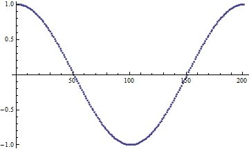
A discussion of Einstein’s reformulation of mechanics would be outside of the scope of this project but the final insight that must be stated in order to fully layout the background of what came to be realized as the electromagnetic field transformations is that the speed of light acts as a fundamental “speed limit” in our universe. This is readily seen by examining the Lorentz factor $\gamma=\frac{1}{\sqrt{1-(v/c)^2}}$, which is ubiquitous in relativistic mechanics. Plotted below, we see that $\lim_{v \to c}\gamma$ diverges, with $v=c$ acting as a vertical asymptote.

With these considerations, that relative motion is the only appropriate lens in which to view the physics between two interacting bodies and that the speed of light–as a law of physics–must be agreed upon by all intertial observers, Einstein derived the famous and familiar length contraction and time dilation formulas, which lead to the electromagnetic field transformations. Although the derivation is simple, it is also long and for brevity I shall simply state the transformations prior to showing their effect on a handful of real world scenarios. Suppose there are electric and magnetic fields defined by the vectors $\vec{E}_x, \vec{E}_y, \vec{E}_z$ and $\vec{B}_x, \vec{B}_y, \vec{B}_z$ respectively, moreover, suppose we are moving throughout space with some velocity $\vec{v}$ in the $x$ direction (this can be assumed without loss of generality as one is always free to define a coordinate system with an axis parallel to their velocity), the relativistic correction to these fields are defined by the following transformations:

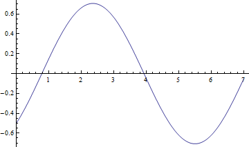
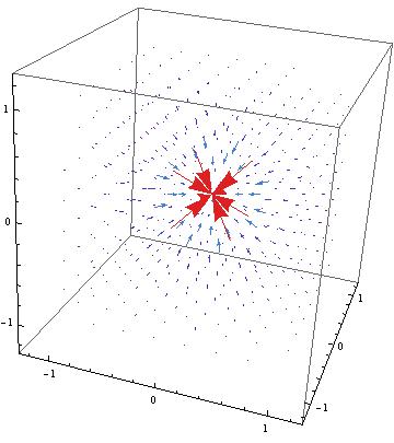
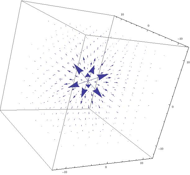
As we’ve seen, electromagnetic considerations influenced the development of special relativity. What is of great interest however is the effect special relativity had in reformulating electromagnetism. Consider the most basic electromagnetic consideration, the field of a point charge, equipotential field lines are plotted below for a stationary charge:

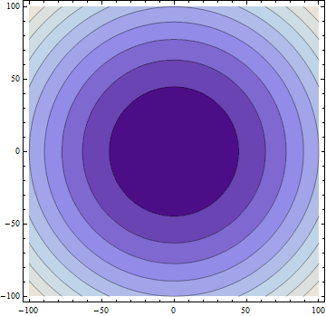
Only cross sections of the field are necessary to observe the physics at play so I’ve opted to obviate the third dimension in this demonstration. In general, the stationary charge can be considered to be surrounded by equipotential circles representing its field. Let $x, y$ represent the horizontal and vertical displacement from the charge in its rest frame. On the surface of any of these circles, the ratio of the field components is equal to the ratio of the displacements, $\frac{\vec{E}_y}{\vec{E}_x}=\frac{y}{x}$.

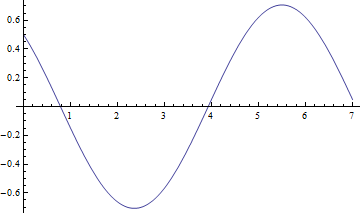
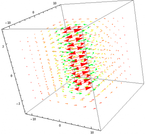
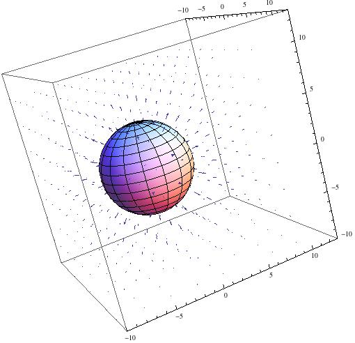
Now let’s think about what we would observe in our own rest frame if this particle moved past us with some arbitrary velocity $\vec{v}_x$. We will observe the horizontal displacement as length contracted, $x’=x\sqrt{1-(\frac{v}{c})^2}$. Moreover, in accordance with the transformations given above $\vec{E}’_y=\gamma\vec{E}_y$, our equipotential surfaces are now parameterized by, $\frac{\gamma\vec{E}_y}{\vec{E}_x}=\frac{y’}{x’}$. For a velocity of 0.9c, we now observe the field to be contracted in the $x$ direction and magnified in the $y$ direction:

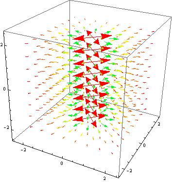
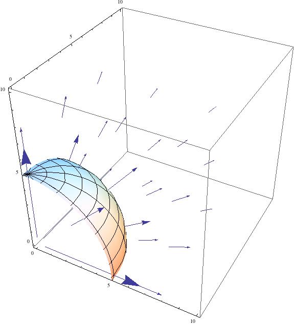
In the limit, setting $v$ infinitesimally close to $c$, we can see that the field in the $x$ direction effectively vanishes:

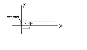
Finally, we will look at one last  enlightening aspect of relativity’s impact on electromagnetism. A common question even among intermediate level students is why exactly a magnetic field of some sort exists. An illustration of “magnetic” forces arising from relativistic considerations–even at low velocity, which we shall explicitly consider–can be seen in the consideration of a test charge moving parallel to a current-carrying wire.  Suppose that the electron current of the wire flows in the negative $x$ direction whereas the test charge and Ben Franklin current both move in the positive $x$ direction. As the wire is electrically neutral, we require both the positive and negative charge densities (ie the distance between two like charges) to be equal. It is fairly easy to calculate the entirely magnetic force in the laboratory frame, where we see the particle in motion relative to the wire: $F_m=\frac{qvI}{2\pi\epsilon c^2R}$ where $R$ is the separation distance between the charge and the wire.

In the test charge’s frame however we will run into a problem if we attempt to calculate an exclusively magnetic force insofar as the magnetic field still exists, but the charge, which is at rest, is incapable of sensing it. That said, there is still a very evident force arising elusively from the relativistic behavior of the wire.

As the charge is moving parallel to the positive current, whatever the speed $v_+$ of the positive charges are will be lessened in the test charge’s frame and thus the length between them will be expanded: $l_+=\frac{l}{\sqrt{1-(v_+/c)^2}}$. Moreover, the velocity of the negative charges will seem to be greater in this frame, thus contracting the distance between them $l_-=l\sqrt{1-(v_-/c)^2}$; where $l$ represents the necessarily equal spacing of the charges in the wire in the laboratory frame.

We can thus define a new charge density, and as $v$ is assumed to be much less than $c$, use the binomial expansion of $l_{+/-}$:

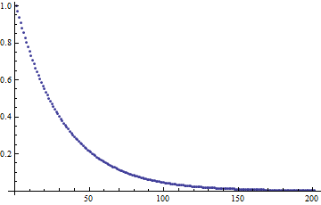
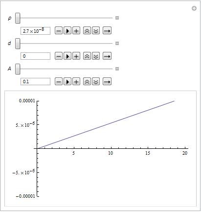
Which is equal to $-\frac{qv^2}{lc^2}$. Plotted as a function of $v$, we see that the density idecreases linearly with velocity within our region of interest:

As current is equal to $\frac{qv}{l}$ we can easily define an exclusively electric force acting on the particle $F_E=\frac{qvI}{2\pi\epsilon c^2R}$. We realize the main computational power of special relativity as it pertains to electromagnetism, the electric and magnetic fields are effectively two components of one unified field, we are generally free to fix a reference frame so that the contributions to the underlying physics can be seen as arising solely from one of the two interactions.

Conclusion: The development of Maxwell’s formal treatment of electromagnetism was pivotal in Einstein’s development of relativity. The contribution was then paid back in full as the relativistic understanding of our universe allows both deep insight and increased computational ability in electromagnetism. What are classically viewed as two phenomena come together in the relativistic view to provide two lenses of looking at problems in which we will always come up with universally agreeable answers.