After some more investigation of our Neural Network model, we have refined our Monte Carlo flipping rules, have stored more than one pattern in our neural network, and have determined that, effectively, the inverse of a certain pattern is equivalent to the initial pattern (they both are energy minima).  Before we delve into these results, we will clear up some questions about our original data post.

Outline:

1. Physics from Statistical Mechanics?

2. A Neural Network

3. Monte Carlo Method

4. Project Goals

5. Constant Energy?

6. Flow Diagram

7. Energy Values

8. Flipping Conditions

9. User Friendly Code

10. Unique Random Pattern

11. J-matrices for A, B,  and their average

1. Physics from Statistical Mechanics?

The model that we are using, the grid of neurons that are either in position +1 or -1, is very similar to the Ising Model (introduced in Chapter 8 of our text), but with some modifications that make it appropriate for modeling brains.  The Ising Model was originally created for studying the magnetic spins of solids and how they interact at different temperatures to explain ferromagnetism vs. paramagnetism, and how those change with phase transitions.  In this model, physics from statistical mechanics is used to see how the magnetic spins interact with a heat bath (temperature is non zero), as well as how they interact with each other: sometimes the spins will flip randomly because of heat bath interactions.  Our neural network model is essentially the Ising model with temperature equal to zero: our neurons never flip randomly on their own, but only in response to their connections with other neurons.  So our model does not use any physics from statistical mechanics, but uses a technique (the Monte Carlo method, which decides whether or not neurons (spins) should be flipped) that is used for many other applications as well.

2.  A Neural Network 

A neural network, in our model, is a grid of neurons (which can have value +1 or -1 only, on or off, firing or not firing), which are completely interconnected (each neuron is connected to every other neuron).  The J matrix is where the connections between neurons are stored, and so the “memory” of the system is contained in the J matrix.  Patterns can be stored in these neural networks, and, if done correctly, stored patterns can be recalled from distorted versions of them.  The way that the neural network travels from the input pattern to the output pattern is via the Monte Carlo method.

3. Monte Carlo Method

The Monte Carlo method is essentially just a way of deciding which neurons to flip, the goal, in this case, being to change the input pattern into one of the patterns that have been stored in the neural network.  The Monte Carlo method checks every neuron, decides if it should be flipped based on certain flipping rules, flips if necessary, and then goes onto the next neuron.  Once every neuron has been given the chance to flip, one Monte Carlo sweep has been done.  The details of the flipping rules depend on the model.  The flow diagram of our general code (in post below) explains our specific Monte Carlo flipping rules in greater detail.

For our neural network, we want to keep doing Monte Carlo sweeps until the output is equal to one of the stored patterns, which is when we say that the pattern has been recalled.  We also want to keep track of how many sweeps it takes to get there, because this is some measure of the speed of the system.  The flow diagram again goes into greater specific detail.

4. Project Goals

Our goal in this project is to investigate the neural network model presented in the text.  First we had to get it working in the first place (meaning we had to be able to store and successfully recall patterns in a neural network), and then we planned on investigating the properties of this model, such as how long memory recall takes for different patterns and different systems, how many patterns could be stored in a single neural network at the same time, how performance of the network changes as more patterns are stored, etc.  How many of these questions we will get to by the end of this project is another story, but we will do our best.

5.  Constant Energy?

The energy of the system, calculated with Equation 12.14 in the text

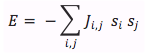
is different for each different state that the system is currently in.  The way that the whole neural network stores patterns is the way that the J matrix is created.  It is created in such a way that the desired stored pattern(s) are energy minima of the system.  Because our Monte Carlo method flips neurons in a way that lowers the total energy of the system, our process should drive P_in towards one of the stored patterns, and stop once it reaches a minimum.  Figure 1 (inspired from figure 12.30 in the text) is helpful for visualization of this energy minima concept, and how stored patterns “trap” the Monte Carlo method and prevent the pattern from changing with further sweeps.  When the Monte Carlo method reaches one of the minima and finds a stable pattern (which is almost always one of the stored patterns, or its inverse (discussed below)), it cannot escape from this energy minima.  If this minima is equal to one of the stored patterns (or its inverse, discussed below), then our code stops and displays the output.  When this happens, we say that our system “recalled” the output pattern.  We also have a condition that stops our code after a large number of Monte Carlo sweeps (1000) and displays the output, regardless of whether or not recall was successful.  This is needed because sometimes the code gets stuck in a shallow energy minimum that is not equal to one of the stored patterns or one of its inverses.  In this case. we want to still display our results and see what went wrong (what pattern our neural network got stuck on).

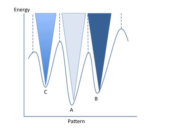
Figure 1: Schematic energy landscape. Each energy minima represents one of the stored patterns. When we give our neural network a specific pattern it produces a pattern with the same or lower energy than the initial pattern.

6.   Flow Diagram

The attached flow diagram provides a step by step guide for our code. This diagram also explains how our neural network functions when performing pattern recognition.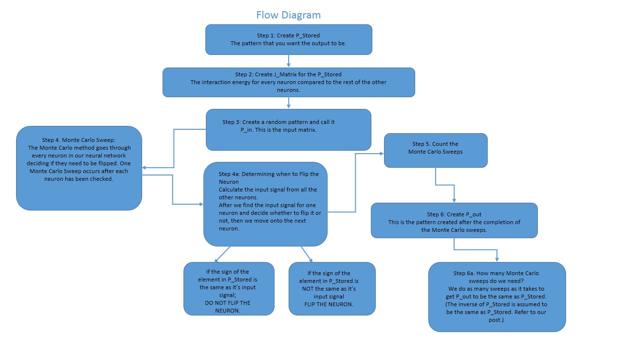

7. Energy Values

We created a code that calculates the energy value for our stored patterns, their inverse, and a randomly generated pattern. Within this code (Energy Calculating Code) you can determine the minimum energy required to flip the neurons from active to inactive or vice versa within our neural network. We want the minimum energy value because this means that our neural network doesn’t need to exert a lot of energy in order to perform pattern recognition.

The energy minima for the stored pattern is much more smaller than that for the randomly generated pattern. This is so because our stored patterns have an order about them that the random pattern lacks. The energy values for the stored patterns and their inverse is -5000.The energy values for the random pattern is always greater than -5000 and close to but never greater than zero.

Furthermore, because the energy minimums are the same for both the stored patterns and their inverses we can assume that the stored pattern and its inverse are the same. In other words, our code starts of with black-blocked letters and the inverse is white-blocked letters. Although, white and black are two different colors, they represent the same letter, due to both of them having identical energies. This phenomenon occurs because if we distort the stored pattern by 80-90% it takes less energy to get to the inverse image than to the proper image, thus the inverse image is displayed as our P_out. In order to avoid this confusion, we set a condition that changes the inverse image back to the proper image.

Link to code: Energy Calculating Code

8. Flipping Conditions

As illustrated in our flow diagram, the flipping conditions determine whether or not the neuron is flipped from inactive to active and vice versa. An input signal is calculated for each neuron and the sign of that input signal is compared to the sign of the neuron. If the signs for both are the same then that neuron is not flipped and remains in it’s current state. However, if the signs are not the same then the neuron is flipped to the state that corresponds with the sign of the input signal.

The input signal is telling the neuron which state to be in. For instance, if the input signal is greater than zero, it is telling the neuron to be in the positive 1 state or if the input signal is less than zero, it is telling the neuron to be in the negative 1 state.

9.User Friendly Code

This code allows for user input to determine which of a variety of input patterns P_in to investigate.  The choices for possible input patterns are listed below (and in comments in the code, if the user forgets):

• P_A and P_B are simply equal to the stored patterns
• negP_A and negP_B are the inverses of the stored patterns
• distP_A and dist P_B are distorted versions of P_A and P_B, distorted by an amount input by the user
• Rand is a random pattern of roughly equal amounts of +1 and -1’s
• Rand_weird (half-way pattern) is a specific randomly created matrix that gets our code stuck, and we don’t know why…

Rand_weird is a specific instance of an input pattern where weird things happened, discussed more in the next section.

Link to Code: User Friendly Code

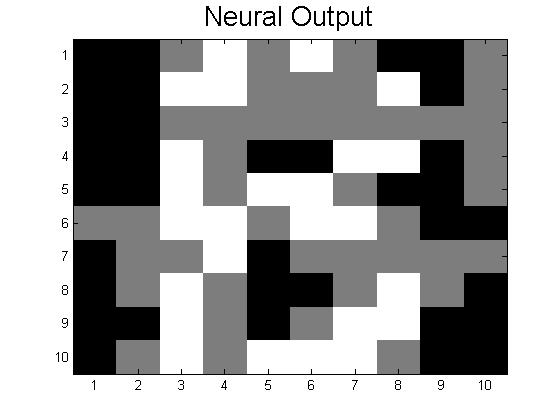
10.  Unique Random Pattern

While we were checking our randomly generated code, we ran into one unique pattern; let’s call it the half-way pattern. The half-way pattern can be assumed to be torn between becoming an A or a B. Because of this, no matter how many Monte Carlo sweeps the half-way pattern goes through, it will forever be torn between the two set patterns. The half-way pattern is the only randomly generated pattern, so far, that has an output where the half-way pattern displayed gray blocks; where the gray blocks represent the number 0. Remember the only two states we have for are neurons are positive and negative one. This gray output has an energy minima of -1745.

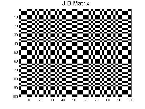
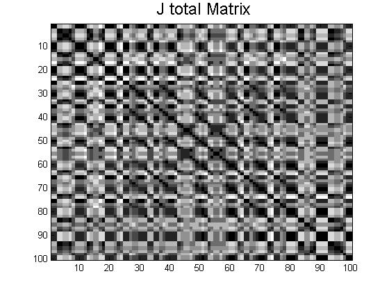
11. J-matrices for A, B,  and their average

Here are the J-matrices created by the pattern A, pattern B and then an average of the two. As you can see there are some patterns within each J-matrix, however it is not a reoccurring pattern. This means that there are certain patterns within each section of each J-matrix.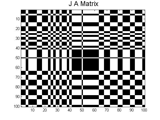       

The piano string is a much more difficult scenario to model than the plucked guitar string.  The guitar string is a pluck, which can be easily modeled with an initial string position.  The piano string has a felt covered hammer that strikes the string, then a standing wave will form.  Seen in the data below, we were able to construct an initial hammer strike on the string, and analyze how it moved throughout:

Our force on the bridge diagram yielded a decent fourier transform but we came across one problem, our hammer string was not executed properly.  In the class text, the force of the hammer on the string, with the spring force behavior from the felt, should yield a soft hit that should appear as a parabolic force vs. time diagram.  Our data shows that it increases linearly and then proceeds to decrease at an acceptable rate. This is something that we must look further into.

Hammer Force seen in class textbook: (Computational Physics, Giordano, p.366)

(image to be added)

Hammer Force we calculated:

This needs to be re-evaluated in order to compare when testing and recording with a physical string.

Link to code: https://docs.google.com/document/d/1tNIwInru6_DcevXB49tW-0ULWkmS8BH2hKv6Tyn9kY4/edit?usp=sharing

Our larger project goal was to  model a three-body system where one object was orbiting a second (larger) one, while an even smaller one was orbiting the first body. The classic example of this system is the earth-moon-sun system.

This second goal was much more difficult than expected considering the relative simplicity involved in reaching the first project goal (simulating the earth’s orbit of the sun). Listed below are some of the different steps that were taken in the direction of this goal. We were not yet successful.

1.

We started out with the entire system: trying to plot the three-body system using the Euler-Cromer method.

And part of it was correct: the earth was orbiting the sun in 1 year. The moon was also orbiting the sun in 1 year. However, the moon was only orbiting the earth 1 time in 1 year, as opposed to about 12 times. Also, according to the program, the radius of the moon was behaving extremely strangely, oscillating sharply between some value for some period of time, then that value would grow a large amount (several orders of magnitude). It would then continue to oscillate.

2.

To confirm the above observation about the moon’s apparent 1 orbit around earth, we changed $dt$ to be extremely small and zoomed in very close to the orbit to examine the moon’s motion more accurately (note the axis in the figure below).

This figure shows that the moon is not orbiting the earth in the correct way.

3.

Our first hypothesis for the incorrect motion was that our initial velocities were incorrect. The image below shows:

Initial velocity of Earth = 2*pi AU/year

Radius of moon’s orbit = 1.0026 AU  (the actual distance)

Initial velocity of the Moon = 2.5 AU

Which was one of our attempts at changing the initial velocities of the bodies. Based off the dramatic responses in the simulation upon changes in initial velocity, we assumed that our hypothesis was either entirely or partially correct.

The next step was to play more with the velocities of the bodies. This resulted in somewhat hectic and clearly incorrect figures. This method was not working as we wanted it to.

Taking a step back, we decided to simplify the system into one that we are more familiar with. Having the “Earth” move in a straight line while the moon orbited it would provide a simpler system to study and model. If we could master this simpler system, it would (hopefully) be easy to shift into a circular motion of the earth instead of a linear one.

4.

Initial distance between the moon (black) and the earth = 1AU

Linear velocity of earth (blue) = 0.1AU/year

Initial x velocity of the moon = 2.4*pi

dt = 0.01

using

(1)  

(2)  

5.

Initial radius of the moon (black) = 1 AU

Linear velocity of earth (blue) = 0.5 AU/year

Initial x velocity of the moon = 2.2*pi AU/year

dt = 0.005

using

(3)  

(4)  

This was becoming a study of how different velocities affect the orbital motion of the two-body system. Unfortunately, the orbit of the moon was not behaving as we wished, even in this simpler program. The orbit began to collapse into itself and the Earth moved too fast for the moon to continue to orbit it. Instead, the moon continued to move in an elliptical motion for some time, but its orbit was completely disconnected from the movement of the moon. Then the orbital motion was lost altogether.

After days of tinkering with the Euler-Cromer method to no avail, we decided to take an even further step back and rethink how to describe the situation of the 3 body system. What might be an easier and more consistent way to describe a circular or elliptical orbit? We decided upon using sine and cosine equations to describe the motion of Earth and the Moon. Although this system brought some of its own problems, mainly programming the system to move, it worked much better than the Euler-Cromer Method and we were able to put all three bodies in the same program. The moon orbit was still slightly unstable, veering off the orbit of the Earth at pi/2 and 3*\pi/2. We determined this was due to the elliptical nature of the orbits, and so specified the major and minor axes of the orbits. This fixed the issue. The problem of actually seeing a body move continues to be a problem, however, as the orbits just look like spinning ovals at the moment. As we continue to work on the program, hopefully we will find a way to represent just a body moving in space with perhaps a thin line to represent the orbit.

All Matlab Codes are listed chronologically (relative to the order in this post) in this Google Doc:

https://docs.google.com/document/d/1-pW6mJHuNV96lPBclSJBbOHwxXdHfXjnpb3cJLJO-30/edit?usp=sharing

It is not the most convenient way to view the codes, but they are color coded to make them easier to look at separately. This was the most convenient way to organize them considering there are so many.

New Resources

1. Williams, Dr. David R. “Earth Fact Sheet.” Earth Fact Sheet. NASA, 01 July 2013. Web. 22 Apr. 2015.
2. Williams, David R. “Moon Fact Sheet.” Moon Fact Sheet. NASA, 25 Apr. 2014. Web. 22 Apr. 2015.
3. “Introductory Astronomy: Ellipses.” Introductory Astronomy: Ellipses. Washington State University, n.d. Web. 22 Apr. 2015.
4. “MATLAB Graphics 2D.” Ku Leuven. Katholieke Universiteit Leuven, n.d. Web. 22 Apr. 2015.
5. Meshram, Ashish. “3D Visualization of SUN, EARTH and Moon.” MATLAB Central. N.p., 16 July 2013. Web. 22 Apr. 2015.

Over the past week I have developed my code to achieve a fairly accurate approximation of Mercury’s precession due to the general relativistic effects of the sun. This was achieved by plotting the orbital motion of Mercury over 7 orbital periods, then saving the locations of the perihelions from each of the orbits. From these perihelions, I was able to graph the precession rate, . For an alpha of 0.0015:

The slope of the linear-squares best fit gives the rate of precession experienced by Mercury at this value of alpha. In order to extrapolate the true precession rate of Mercury (which is very small and would be difficult to calculate using the above method) by graphing the precession rate as would be experienced by Mercury at different values of alpha. (As seen previously, precession rate is given by C*alpha; the relationship between precession rate and alpha should be linear. For Mercury this resulted in the graph:

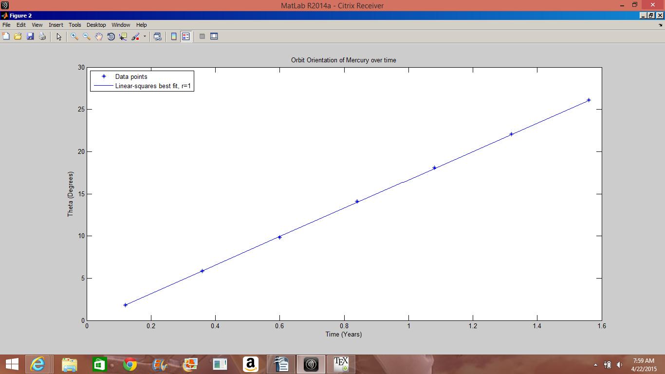
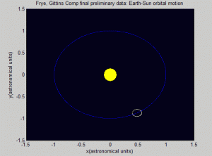
The slope of this graph (C) was calculated to be ; which is close to the true value, . This yielded a precession rate of , as compared to Mercury’s true value, . This corresponds to a percent error deviation of about 10.39.

After completing this extrapolation, I began an investigation into the effect of eccentricity on the precession of the perihelion of a planet’s orbit. I left the both the mass and perihelion values for my test planet to be the same values as for Mercury, however I allowed the semi-major axis length and eccentricity values to vary. Holding the perihelion constant at the value of Mercury’s perihelion results in the expression , where e is the eccentricity and a is the semi-major axis length in astronomical units. Using the same method as given above, I was able to calculate the precession constants C for 7 different Mercurian systems, each with a different value of eccentricity. The results are shown below:

As can be seen by the graph, the best fit for this set of data is a multiple-linear regression fit, of degree 2. Checking this result with Einstein’s expression for the precession rate:

We see that the precession rate is indeed inversely proportional to .

Here is a link to my updated Mercury Precession code:
https://docs.google.com/a/vassar.edu/document/d/1fw8L5ZvhqMMVMYltkJH6Ac425KrmnbbDUJs_6GV7aPI/edit?usp=sharing

And a link to my Mercurian Eccentricity code:
https://docs.google.com/a/vassar.edu/document/d/1eqEBSExnBQZRgFUq9GYQDdjTqC9EODRIR0llXQv7sMw/edit?usp=sharing

References:

Computational Physics by Nicholas J. Giordano and Hisao Nakanishi

Vankov, A.A. “Einstein’s Paper: Explanation of the Perihelion Motion of Mercury from General Relativity Theory”.

The previous presentation of results was very limited–limited in the scope of the actual results that were presented, and limited in the scope of analysis. Here, I present further results with a greater analysis of implications, limitations, etc.

First, let us consider why we care about such a scenario. A sphere is a relatively simple object, but also a very interesting one. Many other objects can be modeled as spheres, or as a combination of several. For me personally, I have been working with a spherical microphone, and since I wish to understand how the sound behaves on the surface of this microphone, I need to take into account how the sound is scattering from the microphone. This is the main practical application I am familiar with, though there are bound to be others.

An acoustic plane wave is very simple and is best shown with an image rather than an equation. Note it is very much like it sounds (no pun intended): a plane (in the mathematical sense) traversing through the air.

Source: commons.wikimedia.org

Now, to understand how this plane wave interacts with a sphere, we need several things: 1) for convenience and simplicity, a way of describing the plane wave using spherical coordinates; 2) a series of functions known as spherical harmonics; 3) and to meet a couple of boundary conditions called the Dirichlet Boundary Condition and the Sommerfeld Radiation Condition.

I won’t go into detail here about 1) and 3), but shall simply show results below. As for spherical harmonics, they are to 3 dimensions what Fourier Series are to 2 dimensions: they allow us to break apart 3D shapes or fields into an infinite series of functions. For more on spherical harmonics, see the end of this post.

The equation describing the pressure field at the surface of a rigid sphere (after being struck by plane wave) is as follows:

Where i is the complex unit, n is a term representing the sum index as well as the spherical harmonic order within the sum, k is the wave-number of the acoustic plane wave, a is the radius of the rigid sphere, m is the degree of the spherical harmonic, Θ_k is simply the (theta, phi) pair representing the direction of incoming sound, Θ_s are the (theta, phi) pairs of every point at which we’ve chosen to evaluate the pressure field (or the “sampling points”), and Ynm is the spherical harmonic of order n and degree m. Finally, bn(ka) is given by:

where jn and hn are the type one spherical Bessel and Hankel functions, respectively, and the apostrophe (‘) denotes their derivatives. Note that this pressure field is the very solution we want–that is, the equation of very near field scattering and diffraction all in one. In fact, it is actually a superposition of incident energy and reflected energy (for more on this, see reference [1] below.

Now, in principle this first equation is exact; it yields perfect solutions with no errors. In practice, however, we must approximate this solution on several levels:

1. We must truncate the sum in the first equation, as finite computing power only allows finite calculation of spherical harmonics and bn,
2. The Spherical harmonics, spherical Bessel and Hankel functions (jn and hn) must be approximated, as they do not have a simple analytical form,
3. The number of points at which we can evaluate the pressure field on the surface of the sphere must be finite (e.g. would could choose 64 evenly spaces points, or 128, etc.); ideally we could choose infinite points

Our main priority here are bullet points 1. and 3. Matlab does a very good job of approximating the Spherical Bessel and Hankel functions, and the error attributable to them is small in comparison with the other two errors. Let’s discuss points 1. and 3. in detail (they shall be discussed together since they are related):

Let N be the maximum spherical harmonic order, or the maximum order of our sum (replacing the infinity in equation 1).

For small N, there are huge errors in the calculated sound field because the spherical harmonics fail to truly estimate the shape of the sound field. They simply can’t produce the detail fine enough. Let’s illustrate the point graphically. Below are the cross-sectional graphs for N=0, 1, 2, and 10 for the sound pressure field at the surface of the sphere, for a plane wave of frequency 1000 Hz.

Notice how the first few graphs fail entirely to capture the true detail of the sound field, whereas the final graph is quite detailed. Spatial errors of this sort, due to the truncation of the sum of spherical harmonics, are called spatial Aliasing Errors.

Another type of spatial aliasing occurs when we try to examine high frequency sound. Since we only have a finite number of points to work with, higher frequency sound tends (or shorter wavelength) to be harder to model. The reason is this: as the wavelength gets shorter, it begins to approach the distance between our samples (if we’ve chosen 64 evenly spaced points, for example, there is finite distance between each point). Once this happens, we no longer have enough samples to reconstruct the sound field. This behaviour is akin to the Nyquist Frequency and sampling rate: signals with a frequency higher than the Nyquist Frequency simply can’t be reconstructed accurately. Let’s look at this graphically as well. Below are the cross-sectional graphs for N=10, 20, 30, and 100 for the sound pressure field at the surface of the sphere, for a plane wave of frequency 20000 Hz. 128 Sample points have been used.

It’s looking good, it’s looking good… and it fails. We’ve maxed out our capability to model the sound at 20000 Hz, and further addition of spherical harmonics, after a certain point, actually gives us worse results.

So, it was seen in practice that choosing a maximum order of approximately N = sqrt(M)-1, where M is the number of sampling points, was ideal for most cases. Addition of higher orders may lead to frequency related spatial aliasing as shown above, though in practice it has been observed that somewhat higher values of N may (a few orders more) may also be acceptable [3].

Below are graphs for the 2D cross sectional area of the sound pressure at the sphere, and the corresponding sound field around the sphere. Results are shown for octave bands between 100 and 8000 Hz (125, 250, 500,1000, 2000, 4000, 8000), the frequency range most important for human hearing. Number of sampling points and N have been adjusted periodically to improve resolution.

Sound field on sphere:

Contour plot of sound field in vicinity of sphere (x and y axes are simply xy-coordinates in meters):

Notice how, for low frequency (long wavelength) the scattering is actually quite low. This should make a lot of sense physically, since the larger the wavelength with respect to the sphere, the more likely the sound is to simply diffract around the sphere and “ignore” it altogether. On the other hand, for higher frequency (shorter wavelength), the scattering becomes quite large, especially at the front of the sphere. This should also make sense, because the spherical boundary becomes more and more like a flat surface to a smaller and smaller wavelength, and hence reflects sound approximately back in the incident direction. Note too that for high frequency there much less diffraction than for low frequency.

TODO: more in depth analysis of error, especially numerically. Clean up code. Comparison to limiting case of Rayleigh scattering.

—————————————————————————————

NOTE: Here is a table describing the function of the code. Below the table is a link to the updated code, which have vastly improved commenting to facilitate use. I would recommend using rigid_sphere_scat_2D over its 3D counterpart, simply because the 2D is so much easier to visualize, and since the scattering is symmetric, it tells essentially the same info.

Link to code:

https://drive.google.com/a/vassar.edu/folderview?id=0B3UNwnkM9fLrfkRlb05LdEVOTzhCQWRuRHRCVVFjUDJIMHBpWlF2V3ZKd3UwWXNwVWRua28&usp=sharing

Spherical Harmonics [2]:

Note that spherical harmonic order starts at 0, not 1.

References:

[1] http://ansol.us/Products/Coustyx/Validation/MultiDomain/Scattering/PlaneWave/HardSphere/Downloads/dataset_description.pdf

[2] http://mathworld.wolfram.com/SphericalHarmonic.html

[3] O’Donovan et al. Imaging concert hall acoustics using visual and audio cameras.

[4] Li et al. “Fast time-domain spherical microphone array beamforming.” IEEE Workshop on Applications of Signal Processing to Audio and Acoustics. 2007

Alex Molina & Kadeem Nibbs
Computational 375 – Project

GOAL: Week 2: Run simple trial with one-dimensional object in two-dimensional space with air resistance ( varying wind speeds and air densities)

In all track events run/jumped primarily in one direction, wind is an important consideration in athletic performance. In the long jump, and in the shorter sprinting events (the 60m, 100m, 200m, and all of the similarly distanced hurdle races), the maximum allowable tailwind (wind propelling the athlete forward), is +2.0m/s. There is no maximum allowable headwind (wind pushing the athlete back), but at headwinds stronger than -5.0m/s, an event might be postponed. For our latest results presentation, we compared the jump trajectories while varying wind assistance and air density, in each case holding all other variables constant.

Our original goal for the week was to improve our model to have a 3D projectile with limb objects, functions to bend and extend the limbs, and methods to calculate the cross-sectional area and center of the mass of the body depending on the state of the limbs. However, we could not figure out how to implement object-oriented design in MatLab, and we failed to properly define functions in our code, which made our prospects shaky at best. We instead decided to learn what information we could from our current working model.

Our results showed that wind assistance has a major impact on performance in the long jump, as a jump into a 5m/s headwind netted a distance of about 5 meters, a mediocre distance for a male high school jumper, and a jump propelled by a 2m/s tail wind recorded a distance of nearly 25 feet, which is an elite college-level distance. We found that air density had a negligible effect on the jump distance, variations of up to 50% in air density resulted in less than a millimeter difference. This reaffirms what we learned in introductory mechanics, that air resistance is negligible in most cases of projecting motion, the exceptions being when the air is moving, and when the object is moving at high speeds. Air resistance will not significantly affect an athlete jumping at 20mph into still air. This also shows that although air density can be as high as 1.2kg/m^-3 at cities near sea level, and as low at .75kg/m^-3 at cities 5000m above sea level, long jumps performed at any city in the world can be compared because of air density’s negligible effects on performance.

Important Links:
MatLAB code and other essential information can be found at:
https://drive.google.com/open?id=0B6loGd4o7iESfjNoRnVmSjJDNHlabG9qNEJIRmY1Z1JEeS1QNE9rTjlIY2Vqc1NMTWlwdEk&authuser=0

References:
Giordano, Nicholas J., and Hisao Nakanishi. “Chapter 2: Realistic Projectile Motion.” Computational Physics. 2nd ed. Upper Saddle River, NJ: Pearson/Prentice Hall, 2006. Print.

Our Resulting Projectile Motion with Varying Wind Speed:

Our Resulting Projectile Motion with Varying Air Density:

UPCOMING: Week 3: 
Run a second trial with a mass-less two dimensional object in 3-dimensional space. We will more to run two test trials with three-dimensional object in three-dimensional space, each with different body position.

Unfortunately, I was unable to finish hacking the equipment in the laboratory to harvest EMG signals. This is because I do not have access to LabView hardware in my lab yet, and as such am currently unable to read my own surface EMG signals onto a computer. However, the sample signals mentioned previously in the preliminary data proved sufficient to proof this code and derive an understanding of the capabilities of this version of the algorithm. Pictured below is the absolute value of a sample EMG spectra (EMGSample1.mat), which allows a viewer a better understanding of the kinds of trends within the signal easier.

I was successfully able to create a working code that finds the peak amplitudes above a contraction threshold, and the thousands of separate cycle durations distinguished in order for each of the the three states of action in the robotic arm, contracting, holding at a contraction, or resting/ returning to resting. Like the previous iteration of code, this version implements a FFT (Fast Fourier Transform) noise analysis process to help eliminate the primary sources of noise in the EMG signal, 60 electronic noise and low frequency (<20 Hz) vibrations. Although significant, the effects of this noise cancellation is not sufficient to fully extinguish all experimental noise. For this data, I cannot include any further analysis as I do not know the lab conditions from which this data originated. Pictured below a snippet of the raw EMG spectra is shown above that same data after being passed through a rectification process. Although noise is still an issue in the rectified signal, the rectified data is more workable than its predecessor. However, since a Fourier transform is a frequency analysis tool, I have had to abandon running a truly continuous analysis in favor of chopping the data up into smaller bins of some small time and going through the analysis process for each bin individually as a quasi continuous process.

For the purposes of testing the efficacy of the EMG analysis code, the noise threshold, which determined whether the arm would be in the resting state or holding some strained state, was made lower than it ought to be in a practical experiment. Similarly, the threshold that determines when the signal indicates contraction was lowered, such that there would be more opportunities within each signal to evaluate if the code was executing as intended. The data for both peak amplitude and cycle duration is saved in a 20 by j matrix, where j is the number of bins that characterizes the stagnant code in this iteration, or in a later version the number of bins that have been created up to this point.  For cycle duration, the data is stored for each bin as a column vector in a matrix, with elapsed time for contraction cycles, rest cycles, and holding cycles stored in order (values 0-1 contraction, 1-2 holding, 2-3 resting). Similarly, the values for peak amplitude during the contraction cycles are stored with the same indices as the contraction duration that they occur during. The peak amplitudes are represented as a proportion of the contraction threshold, which will allow for easier programming of the robotic arm downstream.

The data sets are inordinately large, so I will leave it to the discretion of the reader to use Google drive to access the code and run the results. However, the image below is a screenshot of the results for cycle durations of the first data set (SampleEMG1.mat) between 1.85 and 2 seconds. Although this code serves its purpose, it is not a perfected or completely stable arrangement. Due to the large datasets and indexing method used, changing noise threshold outside of a small range around .1 can or altering the algorithm that controls the analysis can cause the code to crash.

Furthermore, as a byproduct of ensuring a higher degree of stability such that the code is reasonably likely to function properly over a dataseries, the cycles are trimmed slightly and lose resolution in each bin. To compensate for this, any excess time in each bin that has not been accounted for is said to be a hold state at the end of the bin. Though this may seem inefficient, This extra time at the end of each bin will allow the physical system and computational analysis to stay at pace with one another, as the extra hold time can be reduced while the physical system tries to continue a motion. Further work on this code will include making it more robust and resilient, as well as finishing on getting my own EMG signals to analyze. Outside of the context of this class, I plan on integrating the analysis code with the code to control the robotic arm, as well as increasing the sophistication of my model such that the outputs and conclusions better correlate with physical action in a biological agent.

Relevant Files can be found through the link below with headers:

1: EMG_Data_Analysis_422.m

2: SampleEMG1.mat

3: SampleEMG2.mat

4: SampleEMG3.mat

https://drive.google.com/drive/#folders/0B0K4JjJfDy1ffkR4eEZaMzlxb0xvTjRjWDBIUm9iVzZuRmVyeG1aM0RhWHMxcVB6RXZDUFk

References:

1: De Luca, C. Gilmore, D. Kuznetsov, M. Roy, S. Filtering the surface EMG signal: Movement artifact and Baseline noise contamination. Journal of Biomechanics (January 5, 2010) 1573-1579

2: Richards, C. Biewener, A. Modulation of in vivo power output during swimming in the African clawed frog. Journal of Experimental Biology 210 (2007) 3147-3159

3: Lichtwark, G. Wilson, A. A modified Hill muscle model that predicts muscle power output and efficiency during sinusoidal length changes. Journal of Experimental Biology 208 (2005) 2831-2843

4: Computational Physics by Nicholas J. Giordano and Hisao Nakanishi

Nadav Hendel & Matteo Bjornson

Week Two

The celestial two body problem can be solved exactly, allowing us to observe Kepler’s Laws in action, but the same is not always true of the three-body case. Thus, solving the three body problem exactly has been a central problem of celestial mechanics. In this section, we model the effect of adding a third planet into our system. We will use Jupiter, since it has the largest mass of the planets and therefore would have the most significant effect on the Earth and Sun. The planetary motion will still be related using the inverse square law for gravitational force, and the sun will still be fixed to the origin for our first routine Jupiter-Earth.

Jupiter-Earth is very similar to our first routine Planets, in terms of methodology. For each time step, the planets positions are calculated using the Euler-Cromer method. This is completed by keeping track of the distances between both planets and the sun, as well as the interplanetary distance. From these distances, we can compute the acceleration of each planet as related by the inverse square law, and from there, the new positions. The code for this program is quite dense, and as noted in the textbook, it can be more efficient to define some recurring variables at the beginning of the code such that they need not be recalculated during each iterative loop. Despite this we opted not to do this in our code for the sake of clarity since this added efficiency is quite small.

From our initial results running this program, we can see that using normal masses for Earth and Jupiter, stable planetary orbits can be achieved. At this point, we will continue our experimentation by observing how a change in Jupiter’s mass would affect the Earth’s orbit. As an initial point of reference, a small increase of ten fold of Jupiter’s mass yields negligible results, as Jupiter’s mass is still dwarfed by that of the sun.

In the textbook, a mass increase of 1000 fold is supposed to yield much larger changes in the earths orbit. Unfortunately, we were not able to achieve this result exactly, and were only able to note significant changes using a mass of closer to times 9000 Jupiter original mass. The results of this are shown below:

The fact that we had to increase the mass of Jupiter to 9000 to observe noticeable changes in earth’s orbit indicates that we may  still have some bugs in our code that need correcting. According to Giordano, these effects should have been visible at 1/10th that mass.

Now that we have established this model, we also wished to explore what a true-three body system would look like with our second routine. As the mass of Jupiter approaches that of the Sun, or at the very least significant in comparison, it is unreasonable to simulate this system with the Sun fixed at the origin. The difference between the 3-Body Orbit  routine and the Jupiter-Earth routine is that the center of mass is now set as the origin, and we also incorporate the movement of the sun as it is affected by the enlarged mass of Jupiter. The Sun is given an initial velocity so the net initial momentum is zero, keeping the center of mass from leaving the origin. A few interesting things can happen to this system when the initial conditions are adjusted.

The first change we attempted to make with the model was to establish a base case, simply by multiplying the mass of Jupiter by 100. An increase of mass of this magnitude was intended to perturb earth and the sun, but not by much. As you can see below, this change actually had significant effects on both the sun and Earth’s motion. Despite this, the Earth’s motion with respect to the sun still appears very regular.

One of the first things we noticed was extreme sensitivity to initial conditions. In the following two gifs, the mass of Jupiter is multiplied first by 710x, and second by 710.2x. As you can see, this difference of .2 yields a largely different path for the Earth. In fact, it seems that the results from this section are much closer to the chaotic regime than expected due to their sensitivity. This observation might have some insight into why these systems are so hard to calculate in general.

In exploring the effects of different initial conditions, we set the initial velocity of the Sun to zero. We observed the Sun to follow a cusped path, which seemed almost unnatural. Is this even possible? This also made us realize we need to establish a deeper understanding of the implications of giving the Sun an initial velocity.

These investigations have revealed another discussion we were not expecting to find: how do we know these simulations are correct? Or, how do we know the effects we are observing are not artifacts of the numerical approximation or specific lines of code introducing error? Looking forward to next week we need to investigate ways we can can validate our code and results in order to find them meaningful. It is important to have a fundamental understanding of the underlying physics relating to a theoretical model otherwise there will be no intuition regarding the correctness of the outcome. Our initial exploration of these models yielded powerful results, yet we hope to finalize this project by reaching a greater conclusion about the nature of computational approximations of multi-body systems.

Click the two Matlab Icons below to download the Jupiter-Earth and 3-Body Orbit routines:

3-Body Orbit

Jupiter-Earth

Instrument Background

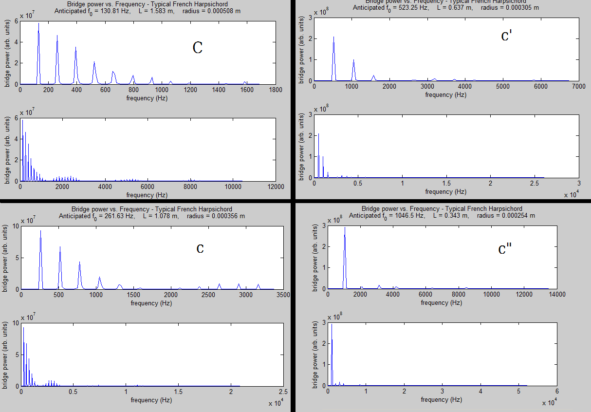
This week’s work comprised of researching the various physical parameters needed as input for the model, which for the harpsichord is functioning properly. I initially believed that there might be a better way to describe the pluck wavefront on the string than simply two straight lines starting at zero at the edges at and in the middle, at some midway point, at . However, this model, used in the book for the guitar, is physically accurate for the harpsichord as well, as both are plucked via a simple mechanism which, unlike the piano, does not impart a time-varying initial force, but rather a simple lift-and-release:

Figure 1: Diagram of the harpsichord’s plucking mechanism (own work).

I simulated the bridge power spectra of four notes from the range of a typical harpsichord: C, middle c, c’, and c”. However, the wire materials used in a typical instrument vary depending on the range of the note sounded; usually red brass is used in the lowest bass, yellow brass in the tenor range, and iron for the rest (Beebe). These different materials, naturally, have different densities, which play an important role in calculating the tension of the string (an input parameter that cannot be directly measured with any ease).

Calculating Tension

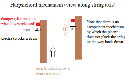
Begin with the equations for the fundamental frequency  of a vibrating string (which defines the note sounded; the quality of the sound is dependent on the strength of specific higher harmonics that also sound):

where  is string length,  is tension, and  is the total mass of the string (Vibrating String). More useful to us is the string’s volumetric mass density  :

where  is the (very small) radius of the wire. These equations can be combined to give:

Armed with an expression for tension containing only known values, the simulations can be run. Note that length, density, and radii data can be found in the bibliography (Di Veroli)(Rose)(Metals and Alloys)(Beebe).

Results

Using the following parameters (some of which are from bibliography, cited above, while others were from personal measurement), the bridge force spectra were computed:

Graphical representation of the fft’s of the four bridge force spectra computed (shown each at two different scales):

Figure 2: Force spectra for harpsichord strings given parameters above. Please click on image to view; any size other than full screen is illegible (hence why it is not full screen here).

Note that the waves in this model do not decay with time; this is a choice in the model and should not strongly effect the outcome, as the intention of the model is to simulate the harmonic frequencies immediately after the initial pluck, not the long term evolution of the system.

As the strings become shorter, the plucking point moves closer to the center of the string, changing the plucking ratio and altering the character of the sound, as indicated by a lack of abundant higher harmonics in the shorter strings (right two figures). This is in agreement with a qualitative understanding of the instrument; bass notes tend to have a more unique sound compared to the high notes.

Further, using the sound function in MATLAB to play back signals produces a very encouraging result: the sound generated purely by this computational model does, in fact, sound like a harpsichord. A further step of the project, analyzing data from the instrument itself, will tell whether or not the model is in quantitative agreement.

The next installment of this project will examine the clavichord, which has a method of sound generation almost unique among musical instruments, and hopefully will include analysis of actual harpsichord data.

Bibliography:

Beebe, “Technical Library, Stringing III: Stringing Schedules“. Accessed 4/21/2015 at http://www.hpschd.nu/index.html?nav/nav-4.html&t/welcome.html&http://www.hpschd.nu/tech/str/sched.html (see “Hemsch Double”)

Claudio Di Veroli, “Taskin Harpsichord Scalings and Stringings Revisited“. Accessed 4/21/2015 at http://harps.braybaroque.ie/Taskin_stringing2.htm

Malcolm Rose, “Wires for harpsichords, clavichords and fortepianos“. Accessed 4/20/2015 at http://www.malcolm-rose.com/Strings/strings.html

“Metals and Alloys – Densities“. The Engineering Toolbox. Accessed 4/20/2015 at http://www.engineeringtoolbox.com/metal-alloys-densities-d_50.html

“Vibrating String“. Georgia State University, Accessed 4/21/2015 at http://hyperphysics.phy-astr.gsu.edu/hbase/waves/string.html

Code

https://www.dropbox.com/s/l8f3sscmel1qdko/Kachelein_Project_Results1.m?dl=0