Preliminary Data

Measuring and Modeling Physical RCL Circuits

Extended Derivations of LC and RLC circuit behavior.

To derive the equations governing the voltage across the capacitor I start with Kirchoff’s Loop Law:

$\Delta V_{L}+\Delta V_{C}=0$ (1)

Substituting in for the values of voltage across a capacitor and inductor we get:

$L\dfrac {dI\left( t\right) } {dt}+\dfrac {Q\left( t\right) } {C} =0$ (2)

The current can be expressed as the rate of change of charge on the capacitor:

$I\left( t\right) =\dfrac {dQ\left( t\right) } {dt}$ (3)

$L\dfrac {d^{2}Q\left( t\right) } {dt^{2}}+\dfrac {Q\left( t\right) } {c}=0$ (4)

This expression is analogous to the equations governing Simple Harmonic Motion (SHM):

$F_{spring}=-kx$ (5)

$F_{net}=ma= m\dfrac {d^{2}x\left( t\right) } {dt^{2}}$ (6)

$m\dfrac {d^{2}x\left( t\right) } {dt^{2}}+kx =0$ (7)

The solution to this second order differential equation can be written as.

$x\left( t\right) =x_{0}\sin \left( \omega _{0}t-\delta \right)$ (8)

Similarly the general solution for charge across the capacitor can be given by:

$Q\left( t\right) =Q_{0}\sin \left( \omega _{0}t-\delta \right)$ (9)

Thus the Voltage across the capacitor, $\Delta V=\dfrac {Q\left( t\right) } {C}$ , can be written as:

$\Delta V\left( t\right)=\dfrac {Q_{0}} {C}sin \left( \omega _{0}t-\delta \right)\left$ (10)

$\Delta V\left( t\right)=V_{0}sin \left( \omega _{0}t-\delta \right)\left$ (11)

RLC circuit (damped oscillation)

The RCL circuit can be similarly derived by adding a third term for the voltage across the resistor to Kirchoff’s Loop Law.

$\Delta V_{L}+\Delta V_{R}+\Delta V_{C}=0$ (12)

$L\dfrac {d^{2}Q\left( t\right) } {dt^{2}}+R\dfrac {dQ\left( t\right) } {dt}+\dfrac {Q\left( t\right) } {c}=0$ (13)

$\dfrac {d^{2}Q\left( t\right) } {dt^{2}}+\dfrac {R} {L}\dfrac {dQ\left( t\right) } {dt}+\dfrac {1} {LC}Q\left( t\right) =0$ (14)

Here we define

$\dfrac {1} {LC}\equiv \omega _{0}^{2}$ and $\dfrac {R} {L}\equiv 2\beta$ (15)

To simplify our second order differential equation to:

$\dfrac {d^{2}Q\left( t\right) } {dt^{2}}+2\beta \dfrac {dQ\left( t\right) } {dt}+\omega _{0}^{2}Q\left( t\right) =0$ (16)

Again, this equation is analogous to Damped Simple Harmonic Motion, described below:

$F_{spring}=-kx -b\dfrac {dx\left( t\right) } {dt}$ (17)

$F_{net}=ma= m\dfrac {d^{2}x\left( t\right) } {dt^{2}}$ (18)

$m\dfrac {d^{2}x\left( t\right) } {dt^{2}}+kx -b\dfrac {dx\left( t\right) } {dt} =0$ (19)

The general solution to this differential equation, describing an underdamped system (where $\beta < \omega _{0}$ ), is as follows:

$\omega _{1}\equiv \sqrt {\omega _{0}^{2}-\beta ^{2}}$ (20)

$V\left( t\right) =V_{0}e^{-\beta t}\sin \left( \omega _{1}t-\delta \right)$ (21)

This solution describes a sinusoidal function whose amplitude decays as a function of $e^{-\beta t}$ .

While in theory my experimental setup is an LC circuit, and should be described by SHM, in reality there should be some form of resistance in the circuit, causing the oscillations to decay over time as described in Damped SHM.

Experimental Setup:

EM-schematics

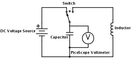
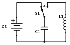
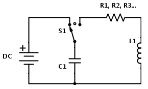
The above diagram represent the physical circuit I built to observe the voltage oscillations of an LC circuit. This circuit has two functions. The first, when the switch connects the loop to the left, charges the capacitor with the voltage source. The second, when the switch completes the right loop, discharges the capacitor through the inductor. The right and left loops are independent of each other because of the switch. Connected in parallel across the capacitor is the PicoScope. This device records the voltage across the capacitor over time. Below are photographs of what experimental setup actually looked like:

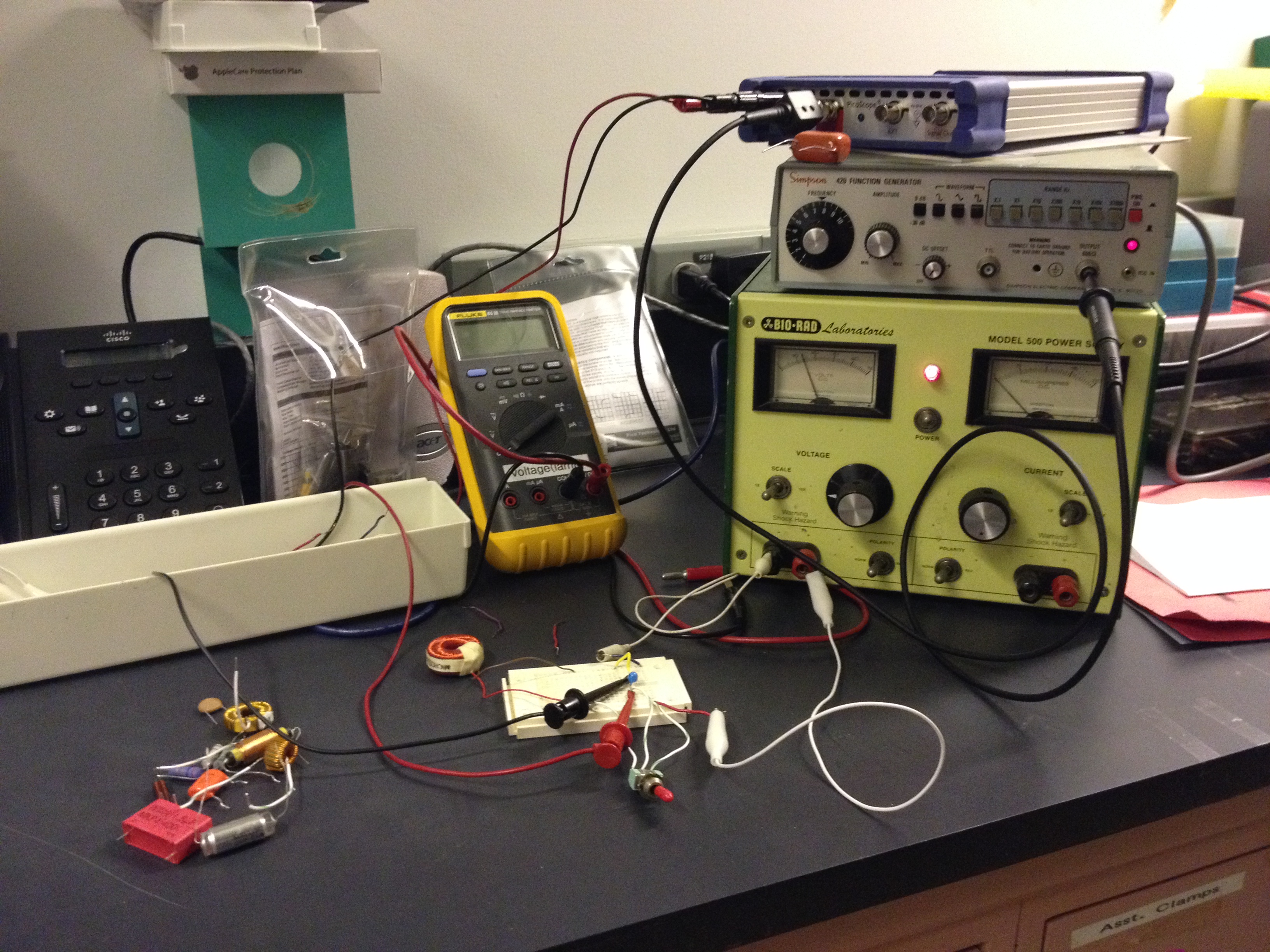
DC power source, signal generator, oscilloscope, circuit (and multimeter).

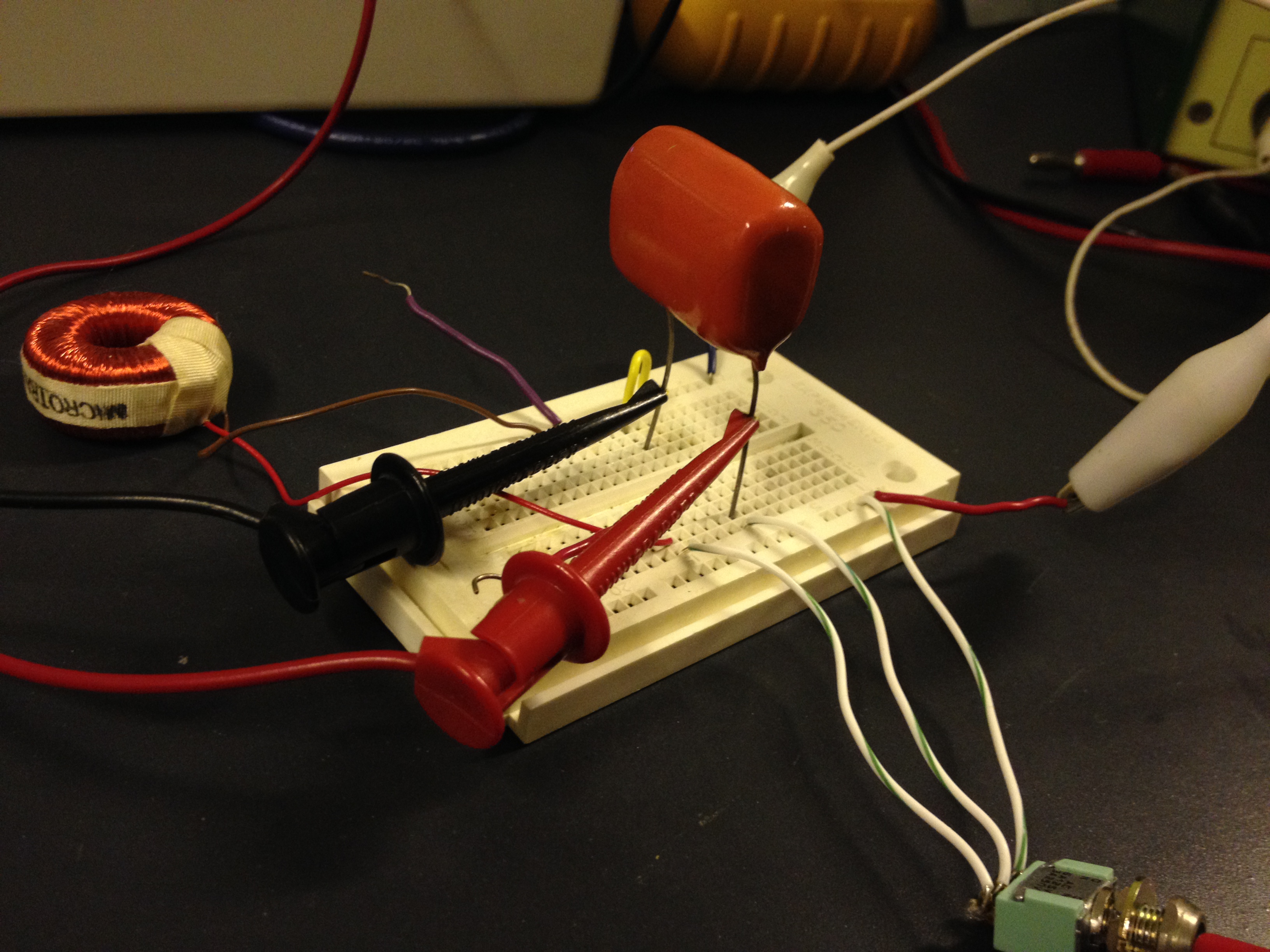
Circuit setup. LC circuit with DC power source, switch, capacitor, inductor, and oscilloscope.

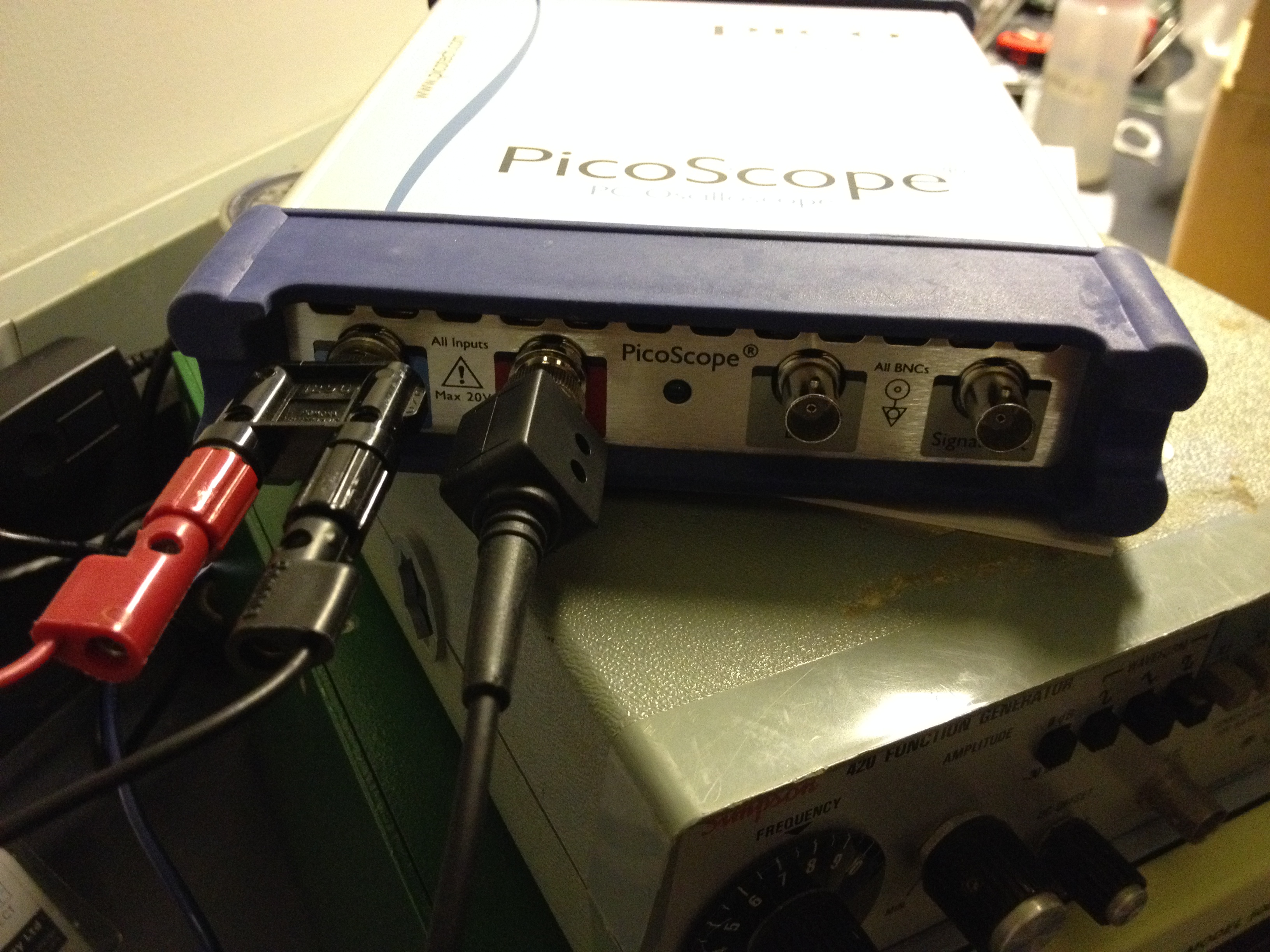
Oscilloscope with Channel A: Voltage difference, Channel B: reference signal.

First Data:

This project held a few challenges of its own before I even got to collecting data. Completely unfamiliar with the Picoscope (digital oscilloscope) probe and software, it took me a few days to figure out how to efficiently collect data with the setup.

My first attempt at taking data did not go well. With the oscilloscope I could see the voltage difference across the capacitor that I wanted, but when I switched the circuit to discharge the capacitor, the voltage dropped to zero immediately. I was looking for some sort of sinusoidal curve, possibly decaying very quickly (in ideal conditions the curve would never decay).

Searching for answers as to why I wasn’t seeing anything, attempted to estimate how long any capacitor would take to discharge.

The charge on a capacitor as a function of time (in an RC circuit) is given by $Q=Q_{0}e^{-tk}$ , where $k=\dfrac {1} {RC}$ . At the time I was using components of unknown value. I visited Larry Doe’s workshop in Blodget and measured the resistance, capacitance, and inductance values of all my components. The capacitor I had picked for my initial measurements had a value of 0.1 μF. What this means is the charge on the capacitor had discharged $e^{-1}$ of it’s initial value (about 37% of it’s initial value) at $t=RC$ . In this scenario the R is the resistance of the circuit. Using an estimation of 0.0001 Ω for 5 cm copper wire as the equivalent resistance of the circuit, and 10^-7 F as the capacitance, the charge on the capacitor should reach one third it’s initial value in 10 ps. To me this illustrated the incredibly short time period at which that particular LC combination would oscillate, and potentially decay.

Second Attempt:

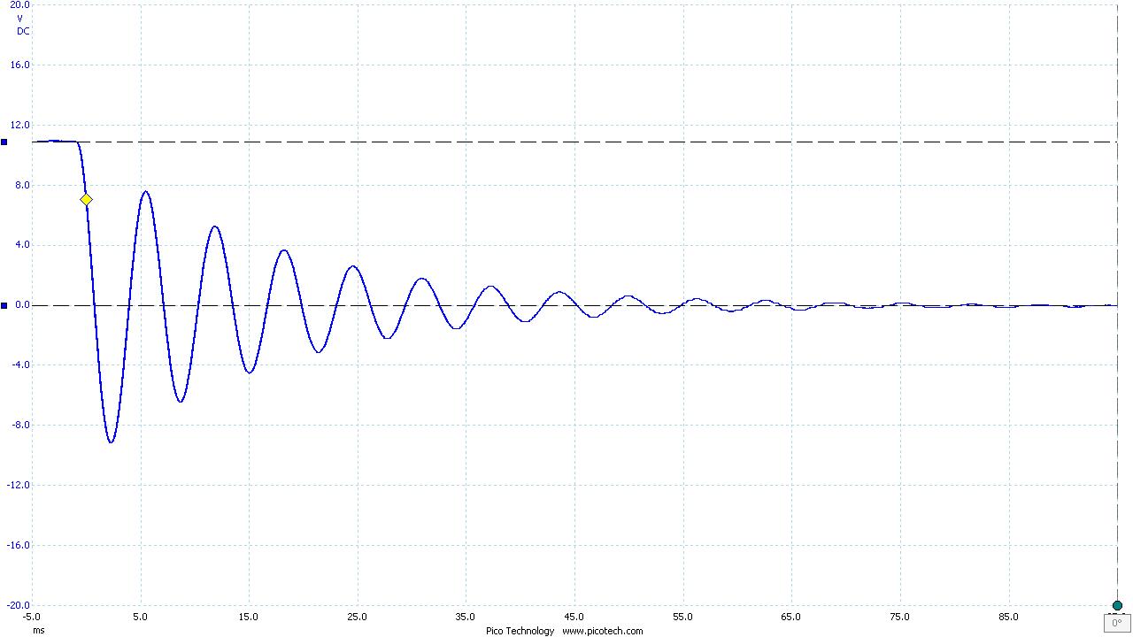
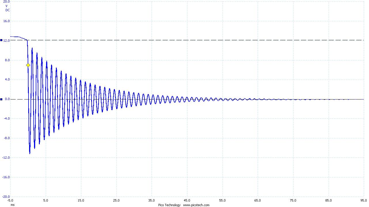
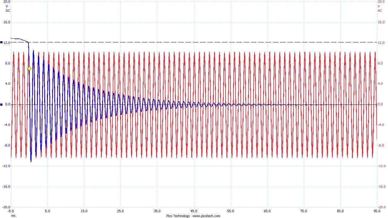
To maximize the time it took the system to discharge I used the highest valued capacitor and inductor I had. The resulting curve was far more manageable. Below is the data I collected with the oscilloscope. The blue curve you see is voltage across the capacitor as a function of time. The total time shown for each image is 100 ms. The red curve is an artificially generated curve for reference. It represents the expected shape of the blue curve. In an ideal LC circuit there is no resistor, and thus no decay over time. Theoretically an ideal LC circuit would oscillate indefinitely.

Figure 1. Capacitor: 1465 nF Inductor: 996 mH

1465nF, 996mH, Oscillation: 128 Hz

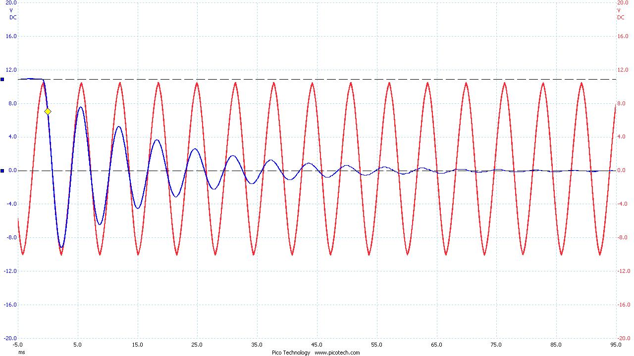
Figure 1.1 With reference wave

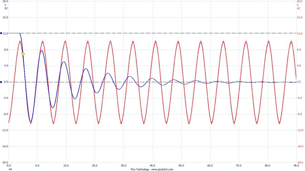
Oscillation: 128 Hz

I then used successively lower and lower capacitor values to approach my initial test where the capacitor discharge was far too quick to measure. The duration of measurement, initial voltage across the capacitor, and inductor value were held constant.

Figure 2. Capacitor: 1007 nF Inductor: 996 mH

1007nF, 996mH, Oscillation: 155 Hz

Figure 2.1 With reference wave

Oscillation: 155 Hz

Figure 3. Capacitor: 47 nF Inductor: 996 mH

47nF, 996mH, Oscillation: 730 hZ

Figure 3.1 With reference wave

Oscillation: 730 hZ

Figure 4. Capacitor: 1.9 nF Inductor: 996 mH

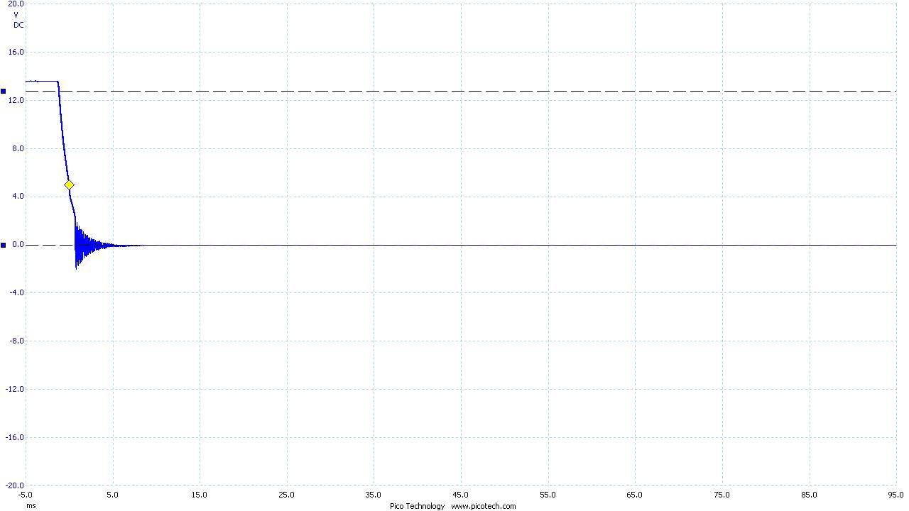
1.9nF, 996mH, Oscillation: 4.23 kHz

Figure 4.1 With reference wave

Oscillation: 4.23 kHz

Conclusion: Electric Fields of Spherical Objects

Gauss’s Law is a powerful tool for understanding electric fields for all types of configurations. The most general case of Gauss’s Law is given by $ \oint \! \textbf{E} \cdot \mathrm{d} \textbf{a} = \frac{1}{\epsilon_0} Q_{enc} $. In this equation, $ \textbf{E} $ represents the electric field vector, $ \mathrm{d} \textbf{a} $ represents the differential area vector of the Gaussian surface through which the electric field is pointed, $ \epsilon_0 $ represents the permittivity of free space, and $Q_{enc}$ represents the charge enclosed by a Gaussian surface.

As stated in my project plan, the general case can be used to solve for the electric field of a point charge, which is given by $\textbf{E} = \frac{1}{4 \pi \epsilon_0} \frac{q}{r^2} \mathbf{\hat{r}} $. The unit vector indicates that the electric field for a point charge points in the radial direction. In my project, I managed to use this equation to model the electric fields for both positive and negative point charges.

I also worked to model the electric field for hollow spherical conductors. The above equation still holds, but with one caveat:

$\begin{displaymath} \textbf{E} = \left\{ \begin{array}{lr} 0 & : r \leq R\\ \frac{1}{4 \pi \epsilon_0} \frac{q}{r^2} \mathbf{\hat{r}} & : r > R \end{array} \right. \end{displaymath}$

In the above, $R$ represents the radius of the sphere. This piecewise function describes the fact represented in Gauss’s Law that a electric fields only exist in regions in which a charge is enclosed. In conductors, all of the charge exists at the outer surface, so there is no electric field on the inside of a hollow spherical conductor. When the distance away from the conductor is greater than its radius, it obeys the second piece of the piecewise function.

This image shows the electric field produced by a positive point charge in free space.

My project was initially intended to be a project that produced visualizations of the above equations. From that point, I intended to develop more complex systems, work out the math for them, and then visually model them as well. However, due to my inexperience with Mathematica 9, I encountered many issues. The RegionFunction proved to be my saving grace, as described in my results post, but it happened too late for me to be able to model more complex systems.

This image shows the electric field produced by a negative point charge. Compare to Figure 1.

This image shows the electric field produced by a negative point charge in free space. Compare to the figure for a positive point charge.

My results do show good visual models for electric fields of single positive and negative point charges, and a positively charged spherical conductor. These visual models are incredibly useful tools for understand electric fields. Looking at an equation (Gauss’s Law) can only do so much for one’s understanding; a visual strongly aids this.

This shows the electric field produced by a spherical conductor with positive charge on the surface.

This shows the electric field produced in free space by a spherical conductor with positive charge on the surface.

I wish that Mathematica had even more tools for visually modeling these electric fields. I tried to create an animation that showed the graphing of the vector field arrows coming out of the point charge, but this did not work. I don’t believe Mathematica’s VectorFunction3D works with its Animate function, but it may just require different inputs. I also tried to create a Manipulate object to demonstrate changes in the electric field as charge changed, but this was also not successful. Part of me believe this is an issue of scaling the image, and part of my believes that this function is also not compatible with VectorFunction3D.

In the future, this project could be expanded by modeling more complex systems. One way to complicate this would be to introduced additional spherical conducting shells with charge on them. Another complicating factor would be to put a point charge inside of a spherical shell. These systems could be modeled with differing signs and values of charges. Additionally, an infinite charged plane could be added to show other ways the electric field might change.

Additional investigations could also include modeling the electric fields of dielectrics instead of conductors. This analysis would be especially complex because it would include polarizations and bound charges. Additionally, this could include the modeling of the electric displacement in addition to the electric field.

Sources and Resources:

Introduction to Electrodynamics, David Griffiths, 4th Edition
Mathematica 9: Student Edition, created by Wolfram
Collaborators: Brian Deer and Tewa Kpulun

Van Allen Belts Modeling – Conclusion and Final Thoughts

At the conclusion of this project I have to say I came out of this project having learned a lot about organizing a project, the Van Allen Belts and how to work with Mathematica. But first I would like to discuss the conclusions that can be drawn from my final data.

Unfortunately I can’t draw any major conclusions about the Van Allen Belts and their location depending on core size as I was not able to incorporate that particular information into my models. I was however successfully able to model the vector fields of a magnetic dipole using Mathematica and an initial equation given by our textbook, a task that proved to be difficult enough on its own to figure out. In the end I did prove that the equation was valid and created a vector field that resembled the expected field of the dipole. Even with this however, I question the validity of the models that were obtained using Mathematica. As I mentioned in my “Final Data” post, the vectors do not seem to vary with respect to the radius away from the origin which doesn’t match the actual system I was attempting to model. It should be decreasing with respect to distance. In the end the project was never really able to combine the Van Allen Belt mapping and the modeling of Earth’s magnetic field into the single cohesive unit.

Furthermore the model itself had a lot of assumptions that needed to be put into place in order to make it easier to develop or simply because I could not figure out how to account for it within Mathematica. The assumptions were listed throughout my final data but they included using a constant magnetic field isolated from the sun’s solar wind to model out the Van Allen belts and assuming the Earth to be a sphere. In the long term however, these were all reasonable assumptions in astronomical scales.

If there was one thing I was somewhat disappointed about, it was the learning curve to reacquaint myself with Mathematica. It had been awhile since I had used Mathematica and it took some time to recall the best functions to use for particular tasks. Furthermore when trying to learn how to do a new task; like converting between Spherical and Cartesian coordinates with Mathematica, it was a long process of trial and error to achieve a result you were looking for. More often than not you would get something more like this:

No Mathematica...this isn't rotating my graph...good try though.

Occasionally, the program has a cruel sense of humor

So a great deal of the project was spent playing around with Mathematica more that playing around with the physics. I do certainly wish I had a bit more time to play around with the physics and even more time to play with the Mathematica program. After a few breakthroughs, I was quickly understanding how to make the program much more cooperative and finding relevant information in the help menus faster. With a little more time, I fixed and accounted for a few of the issues that had been plaguing my models.

Regardless, I was a bit overzealous with the scope of my project. It had a lot of components that were much more difficult than I initially expected them to be. What I ended with were two separate projects, a research summary of Van Allen Belts and a 3D model of Earth’s magnetic field with vague notions of where the Van Allen Belts would be located. Still I am proud of what was accomplished. Modeling the vector field of a dipole was a difficult task and a properly organized model was created.in the end. It was also plotted with proper constants though it needed a little tweaking to confirm that the structure was as expected. Finally from this point it could easily be picked up and completed at a later date with those willing to work on it needing only to manipulate the dynamo equation into an easier form.

Final Remarks

In this post, I will discuss the results of the final data, what I learned, and suggestions for further work.

I began by using one of the most fundamental and well known laws in electromagnetism: Gauss’s Law. It allows for the relatively simple modeling of electric fields of various geometries, where the direct formula for the electric field would have been difficult, if not impossible, to use.

I used this law to derive some the electric fields of some more common physical geometries dealt with in undergraduate physics, which the exception of one configuration: the electric dipole. Through this process I not only re-affirmed my knowledge of the principals involved but learned how to communicate them in an effective way. I then used Mathematica to model the derived electric fields to provide a visual representation.

This was particularly challenging as I do not had a significant background with computer programing at all, let alone with Mathematica. From this work I significantly improved my working knowledge and understanding of this software, not only through the programing but through explaining what was being done throughout the code.

The final results displayed how the electric field of the particular configurations of a sphere, cylinder and ideal dipole work and these results agreed with known models. The basic principles showed that electric fields point away from positively charged objects and towards negatively charged ones, which is most clearly seen in the model of the dipole.

Further work with this topic ideally would include the modeling of more complex systems, such as multiple spheres or cylinders of varying charge or charge densities. It would also be interesting to compare the magnetic field configurations of similar objects, which unfortunately was not able to be done as originally planned due to limitations of Mathematica and available working material.

Van Allen Belt Modeling – Final Data

Background Information:

Earth’s Van Allen Belts are a naturally occurring phenomena due to the presence of the Earth’s magnetic fields. Specifically, they are two zones of space where large concentrations of high energy particles are trapped by the magnetic field lines of our planet. The zones are defined by our field lines; toroidal in shape, and encompass the planet at particular radii from the surface. Following the field lines, the regions begin from Earth’s Southern Pole and loop to its Northern Pole This is illustrated in the diagram below.

Cross-Section of the Van Allen Belts

The particles of these regions include fast moving electrons,and ions from the solar wind along with protons and other remnants of cosmic ray interactions with our atmosphere. All of these particles are electrically charged and thus their motion becomes highly constrained as they pass through our magnetic field; or magnetosphere. As they interact with our magnetic field lines, a force is exerted and influences their direction of motion. It attempts to make the particles rotate about the lines rather than allowing them to continue drifting in a straight line. Thus “sliding” begins to occur; the particles gain a spiral trajectory during which they orbit the field lines while vertically moving along them. Since the magnetic field is stronger as you get closer to Earth however the particles will stop and eventually reverse their motion as they approach the poles. This bouncing between the hemispheres establishes the permanent belts.

The constituent particles and stability of the belts however depends on the location.and thus the strength of the magnetic field. The inner belt is compact; ranging only from 1,700 km to 13,000 km above the Earth’s surface. It is made up primarily of high energy protons created during cosmic ray interactions with the atmosphere. Of the two belts, it is the most stable due to the higher magnitude of the magnetic field lines at that proximity to the Earth. While it gains high energy particles at a comparatively slow rate, it holds onto the particles for an extended period of time and reaches a much higher intensity than the other belt.

The outer belt ranges from 20,000 km to 40,000 km from the Earth’s surface and consists primarily of the ions and electrons that make up the solar wind. Due to the weaker magnetic field at that distance from Earth, the zone is tenuous and loses its particles very quickly. The constant supply of particles from the solar wind however means that the belt has plenty of material to be created from, though its dependence on solar wind particles means that its intensity fluctuates proportionally with solar wind activity. With this background information established, the information needed to created valid assumptions was gained.

2D Vector Fields:

Unfortunately, this also marks the point where my project strayed away from modeling the Van Allen Belts to a more general modeling of the Earth’s magnetic field. The initial task of modeling the magnetic field of the Earth was necessary to define the locations of the Belts with specific field lines that would be seen in the vector plot. Now with some research I found that the Earth’s field could be generally modeled as a magnetic dipole oriented with the south end pointed in the positive z direction. This model is a very basic assumption and ignores the effects of the solar wind on Earth’s magnetosphere, however the area where the Van Allen Belts are present does not get severely effected by these factors except in extreme circumstances. This means a model of a dipole will be generally accurate for our purposes. Thus the first task was to create a model of the magnetic field of the dipole.

The equation for the magnetic field of a dipole with respect to the radius was found to be

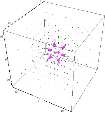
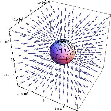
$\vec{B_{dip}}(\vec{r})=\frac{(\mu_0)(m)}{(4\pi*r^3)}(2cos(\theta)\hat{r}+sin(\theta)\hat{\theta})$

This equation was obtained from Griffiths’ Introduction to Electrodynamics. To insure the equation worked I began by applying a constant free version, evaluating only the variables. However, the equation was given in spherical coordinates which Mathematica can’t plot efficiently. To compound that issue, the command CoordinateTransform does not properly evaluate the points which led to several attempts to obtain the proper Cartesian conversion of our equation. Finally, I was able to find the command TransformedField which took into account the variables being used and allowed for a direct conversion. The code and direct conversion can be seen below.

From these equations, I created a vector field of the xz plane with VectorPlot which can be seen below.

Simple vector model of the xz plane of the magnetic field of a dipole

With this successful, I then applied the proper constants to the vector field components and attempted to recreated the field. These constants were the permeability of free space ( $\mu_0$ = $4\pi$*$10^{-7}$ $N$/$A^2$) and the magnetic dipole moment of the Earth ($m_{Earth}$ = $7.79$*$10^{22}$ $A*m^{2}$).The circle in the center of the graph represents the Earth, under the assumption that the Earth has a constant radius of $6.37*10^6$ m.

Model of the xz plane of the dipole’s magnetic field using Earth defined constants

Note that in this plot, the vectors seem to lack the fine structure of the previous field however the vectors are still properly oriented. They continue out from the southern hemisphere and seem to eventually loop back around and end in the northern hemisphere. I attempted a variety of scales and vector size values but no matter what, when the constants were applied to the equation they never had the same shape as the previous vector field. The other concerning aspect of the field was the fact that the vectors don’t seem to weaken as the field continues away from the Earth. It could be that the scale was just off so it was not evident, but even with the shifting of the scales, the vectors still seemed to remain the same size. The general direction and shape was obtained with these equations so I continued on to the next step.

3D Vector Fields:

Applying the same methods as before, I used the vector field components from the obtained equation and using the command VectorPlot3D, I created a vector field of the general equation without the constants. This field can be seen below.

Simple vector model of the magnetic field of a dipole

Without constants the shape of the vector field directly resembles the magnetic field of a dipole in 3 dimensions. Unfortunately, we also have the vectors not varying as expected as the distance from the origin increases. Regardless, after the success of obtaining the proper vector field shape and direction I decided to apply the proper constants to see if the shape would be altered as it was in the 2D graph. The constant applied vector field can be seen below. Once again the constants remain the same and the sphere in the center of the plot represents the Earth, assuming it is a sphere with a constant radius.

Vector model of the magnetic field of a dipole using Earth defined constants

As we can see, the same lack of detail is present when the constants are added to the vector field. However the shape and direction of the vector field are still generally correct though the fine structure is again lost. The vectors still don’t seem to vary with distance as well, which is troubling for actually plotting the field but the model does seem to accurately plot the field itself.

Further Plans:

Unfortunately it is at this point where I ran out of time and needed to call it quits on the project, with only the magnetic field of the dipole modeled. While I will discuss what I would have liked to change and go into more detail on complications within my “Conclusion”, I would like to take a moment to discuss where I wanted to continue on with this project. Specifically, next on the list would have been adjusting the vector field 23 degrees from the z-axis to account for the Earth’s natural tilt. I experimented with a few methods to do this but none of them were truly successful.

Next I would have liked to incorporate a model of the dynamo theory to account for the Earth’s magnetic field. One of the biggest assumptions made within this project was that the Earth’s magnetic field simply existed as a giant bar magnet in the surface. The magnetic field is actually generated by the motion of liquid iron present in the Earth’s outer core. Using this knowledge, I was hoping to create an animation that would allow the observer to alter the size of the planet and then the percent of the outer core took up of the interior. This would allow the observer to have a general model about how the magnetic fields change with different core sizes and thus the location of the Van Allen Belts. Knowing this, scientists could prep future scientific equipment for radiation exposure even if they needed to orbit within the Van Allen belts.

Here are my Mathematica Notebooks in case there were any questions on my code: 2D Vector Fields, 3D Vector Fields, and General Experimenting

Sources:

Griffiths, David, Introduction to Electrodynamics

Stern, David, Radiation Belts (http://www.phy6.org/Education/Iradbelt.html)

Dynamo Theory (https://courses.seas.harvard.edu/climate/eli/Courses/EPS281r/Sources/Earth-dynamo/1-Wikipedia-Dynamo-theory.pdf)

Magnets and Electromagnetism (http://hyperphysics.phy-astr.gsu.edu/hbase/magnetic/elemag.html)

Relativistic E&M: Final Conclusions

While I did succeed in creating a model that allowed the user to view the field at different speeds, it only managed to show the direction and relative magnitude compared to the rest of the current fields. If I were to continue with this project, I would attempt to improve it in several ways.

-First, I would try to find a way to make Mathematica account for the absolute magnitude of the fields so that the uniform fields would appear to change as the speed was varied. This might be accomplished by using equipotential surfaces rather than vector fields.

-Second, I would write code such that the user could simply input (or maybe copy and paste) a particular E-field equation for a rest frame, and the program would interpret the equation and produce the vector plots with sliders as shown in my model.

-Third, I would model more discrete situations rather than infinite distributions of charge or current so that the changes in field would be more visible.

-Fourth, I might consider a different type of plot, since Mathematica seems to deal with this kind of plot poorly. For instance, a static plot of E versus v and B versus v at a single point in space might better show the changing relative magnitudes of the fields.

That being said, this project was successful in several regards. It emphasizes the interplay of electric and magnetic behaviors when considered in moving reference frames, and at least in the case of the point charge, it allows for an examination of the changing shape of the fields at different speeds. It also sets up the framework for being able to model more complex systems by providing a proof-of-concept using simpler cases. Therefore, this project successfully modeled the fundamentals of relativistic electromagnetism, and provides a good foundation for a more in-depth exploration.

Final Remarks

In this post, I will discuss the results of the final data, what I learned, and suggestions for further work.

Magnetic Field Conclusions

When I started this project I initially had the intention to model the magnetic fields due to a cylinder, bar magnet, and sphere. Little did I realize that while I knew that these fields should look like theoretically, modelling them would have been a great undertaking. The fields due to a bar magnet is that of a magnetic dipole and that in itself seemed as though it would have been a project. The sphere could have been modeled in two different ways: as a rotating sphere of charge, or a collection of current-carrying loops. Both were very difficult to find the magnetic field for at any given point and so I was at a loss for things to model.

I was only able to successfully plot the magnetic field due to a line of charge rather than a cylinder since I was having trouble making Mathematica plot piecewise vector functions. The plot below was all that I had to work with.

After some discussion with Professor Magnes, I decided I would take what I had, and make more complicated systems with it.

As seen in my previous Final Data post, I was able to show that if identical current-carrying wires were aligned next to each other, their resulting magnetic field would resemble that of the field due to a plane of current as the distance between them decreases.

The only problem I faced was that I could not find a way to superimpose the vector fields from my aligned wires. While this would have made my model look nicer, it is still relatively clear to understand how the field lines add together.

Next I decided I would use the same method that I used to mimic a plane of current and attempt to model a magnetic dipole. Rather than placing two identical current-carrying wires next to each other, I made one of them have a negative current. I would then plot their resulting vector fields and change the viewpoint such that only the x,y plane was seen.

Again I was faced with the issue of superimposing my two vector fields. However, I suspect that if I found a function Mathematica that would do this for me, I would have indeed modeled a magnetic dipole.

While the topic of my project was by no means a very complicated one, it would be false to say that I did not learn anything from it. My understanding of how Mathematica functions as a program has grown and I have come to appreciate its capabilities. I also learned that while something may seem simple at first in theory, it can be very complicated to achieve in reality.

Conclusions: Capacitors

(Revised 5/7/14)

Initially, I intended to model capacitors of various shapes, including more realistic configurations like rolled-up plates or variable (i.e. adjustable) capacitors. Though these configurations were not ultimately simulated, the information gathered, looking only at square parallel plate capacitors, was illuminating, and the foundational programs I wrote could, with some manipulation, be extended to more complicated arrangements.

The method I ended up using, detailed extensively in the data post, was relatively efficient but still took a non-trivial amount of time (see below) to simulate the electric fields that dictate the properties of a capacitor. The size of grid I used (averaged over two grids: one with 211^2 = 44521 points, the other with 212^2 = 44944 points) was chosen so that the simulated electric fields were at least 99.9% accurate over the distances examined and so that the simulations took no more than 10 minutes each to run (6 plate simulations were run in total, resulting in an hour of pure computation; note that by taking advantage of plate symmetry, this was actually 1/4 the time one might have expected, as it took about 2.4 seconds to find the E-field at any point).

Accuracy of the method at calculating the E-field was checked at a few points against the computationally inefficient but presumably 100% accurate theoretical model, which is based on fundamental physics (integral Coulomb’s law). This method took up to 10 minutes to calculate the E-field at an arbitrary point near the capacitor, though it was much faster far away from the capacitor (where we are naturally not interested).

Splitting a shape into thousands of manageable quantized points charges (each producing a field in accordance with Coulomb’s law for point charges) proved to be an effective tool, even for the relative simple square plates studied here. This method could be expanded in the future to much more complicated surfaces or even volumes to accurately model the electric field of complex shapes that would otherwise be hopeless to analyze analytically. Of course, a real charged object is charged with a finite number of charge carriers, so this method is not physically unsound (on the other hand, a plate charged to 10^-6 C like mine would need 6.25 x 10^12 electrons spread over it rather than a mere 44,000)

It should be noted that I did not examine the effects of dielectrics placed between plates. Though this was originally planned, I omitted doing this not out of time constraints, but rather because it would not have proved particularly illuminating. Linear dielectrics (the only kind extensively analyzed in 341) have very straightforward effects on energy storage and capacitance, which do not seem to depend on capacitor dimensions. Equation 4.58 and an unlabeled equation on page 197 make this clear (Griffiths, 4th ed.):

$W=\frac{1}{2}\int \vec{D}\cdot \vec{E}\text{ } \mathrm{d}\tau,\text{ }\vec{D}=\epsilon \vec{E}$

$C=\epsilon C_{\text{vacuum}}$

Overall, this project was an excellent exercise in computation and matrix manipulation (the data for the electric field at a set of points above a plate was stored in a 3 by 1024 matrix, for example). It was also very useful for practicing using approximation methods based on fundamental physics to solve an otherwise complicated problem. In the end, the ideal model of a capacitor was shown to be insufficient for extremely accurate capacitor parameters at all but the closets plate separations. Of course, real capacitors have by their design very close plates to maximize capacitance, so the choice of method depends on one’s needs and situation.

Perhaps the most useful “next step” would be to take the data for more plate separations and fit a curve to the points, resulting in a function for capacitance or energy as a function of plate separation. Based on the few points I took (see the animation), such a function is approximately a straight line for very small separations (i.e. the ideal approximation) but diminishes with distance like a square root function.

The code used to run these simulations could be expanded upon to use for visualizing electric or potential fields, or for any other application where an arbitrarily complicated electric field (or possibly a gravitational field) needs to be modeled. I tried to keep a neat, albeit very lengthy, notebook file, though I could have labeled my graphics and the computation times more clearly (I used the Timing function on almost every computation, but the way Mathematica returns the timing value is not extremely conspicuous).

Conclusion- Modeling the E and B Fields of A Cylinder

In the beginning, I set out to model the electric and magnetic field of any objects shaped like a cylinder. I wanted to demonstrate the direction and intensity for a conductor, a dielectric, and a coil. I did not get to model the E and B fields for all those different types of cylindrical objects, however I developed a method for modeling on mathematica. With the “Help” tab I was able to model the direction and intensity for a conducting cylinder.

To find the electric field I chose to look at the E and B-fields of a long cylinder first, where this cylinder had a uniform charge density. Using Gauss’ Law I derived the E field (inside the long cylinder) and started looking at different functions on mathematica, to determine which one best demonstrated the direction and magnitude of the electric field. I first converted the coordinates from cylindrical to cartesian using the TransformedField function. After playing around with the VectorPlot and VectorPlot3D I was able to show (using the Show function) the electric field of a long cylinder. The E-field for the long cylinder, from my previous post, demonstrate the electric field within the long cylinder, where the electric field magnitude is directly proportional to the radius of the Gaussian cylinder. So, it makes sense that the arrows are getting thicker instead of shrinking in size.

To find the magnetic field I also chose the same long cylinder, only this time, with a uniform current distributed on the surface of the cylinder. With this induced current flowing in the negative X direction, into the screen, I used the right hand rule to find that the magnetic field is in the positive phi direction. Using Ampere’s Law I came up with the equation for both inside and outside of the cylinder. As you can see in my previous post, the B-field equals zero inside of the cylinder and the B-field outside is inversely proportional to the radius of the cylinder. This is so because all of the current is on the surface of the long cylinder and as you move further away from long cylinder the intensity decreases.

I then used the same procedures, kept the charge density for the E-Field and uniform current for the B-field the same. However, the equations are different now because of the parameters I placed on the finite cylinder. This cylinder has a length of 30cm with a radius of 10cm. After putting that into mathematica, similar results to the long cylinder were produced.

My main focus for this project was to learn how to use mathematica because deriving the E and B fields for a cylinder are things we learn in class. Mathematica is frustrating at first but after figuring out the proper functions I was able to model what we learn in class.

Modeling and Experimental Tools with Prof. Magnes

Ideal for getting ideas and feedback on upper level physics tools.

Preliminary Data

Measuring and Modeling Physical RCL Circuits

Extended Derivations of LC and RLC circuit behavior.

Experimental Setup:

First Data:

Second Attempt:

Conclusion: Electric Fields of Spherical Objects

Van Allen Belts Modeling – Conclusion and Final Thoughts

Final Remarks

Van Allen Belt Modeling – Final Data

Relativistic E&M: Final Conclusions

Final Remarks

Magnetic Field Conclusions

Conclusions: Capacitors

Conclusion- Modeling the E and B Fields of A Cylinder