
When I started this project I initially had the intention to model the magnetic fields due to a cylinder, bar magnet, and sphere. Little did I realize that while I knew that these fields should look like theoretically, modelling them would have been a great undertaking. The fields due to a bar magnet is that of a magnetic dipole and that in itself seemed as though it would have been a project. The sphere could have been modeled in two different ways: as a rotating sphere of charge, or a collection of current-carrying loops. Both were very difficult to find the magnetic field for at any given point and so I was at a loss for things to model.
I was only able to successfully plot the magnetic field due to a line of charge rather than a cylinder since I was having trouble making Mathematica plot piecewise vector functions. The plot below was all that I had to work with.
After some discussion with Professor Magnes, I decided I would take what I had, and make more complicated systems with it.
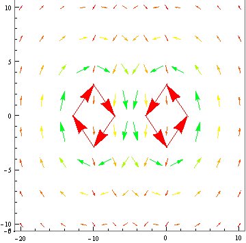
As seen in my previous Final Data post, I was able to show that if identical current-carrying wires were aligned next to each other, their resulting magnetic field would resemble that of the field due to a plane of current as the distance between them decreases.
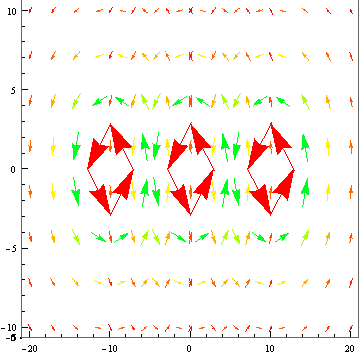
The only problem I faced was that I could not find a way to superimpose the vector fields from my aligned wires. While this would have made my model look nicer, it is still relatively clear to understand how the field lines add together.
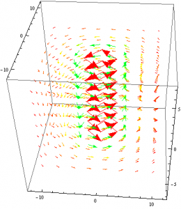
Next I decided I would use the same method that I used to mimic a plane of current and attempt to model a magnetic dipole. Rather than placing two identical current-carrying wires next to each other, I made one of them have a negative current. I would then plot their resulting vector fields and change the viewpoint such that only the x,y plane was seen.
Again I was faced with the issue of superimposing my two vector fields. However, I suspect that if I found a function Mathematica that would do this for me, I would have indeed modeled a magnetic dipole.
While the topic of my project was by no means a very complicated one, it would be false to say that I did not learn anything from it. My understanding of how Mathematica functions as a program has grown and I have come to appreciate its capabilities. I also learned that while something may seem simple at first in theory, it can be very complicated to achieve in reality.

Overall, I think you did a very good job of adapting the project as you worked through it and of discussing why you did what you did/what it means. I think that is very important to be able to do, from the perspective of general problems-soling processes. I also think you did a good job of talking about the implications of your model – specifically how the system of several wires could be expanded to approximate a plane of current.
By the way, I think that Mathematica will add the vector fields if you define a new field which is the sum of two fields. For example, using your names, if the field from one wire was “bCart1” and from the other was “bCart2”, defining “fieldtotal = bCart1 + bCart2” and then using Vectorplot with fieldtotal as the argument should do the trick, I think. At least that’s how I got the field outside the torus of my model to be zero (field1 was the torus, bCart2 was piece-wise defined as negative bCart1 or zero, depending on the location).
Your presentation both in class and on the blog were organized and clear, and your Mathematica file was sufficiently clear and explained. I think the only thing that I would have done differently is to have still compared to Peter’s results, even though your project parameters changed. It would have been a nice followup, and highlight to readers how you adapted to change in your project.
I enjoyed reading it, and I think you did a great job! Thanks!