Using MATLAB, I’ve created several functions to visualize scattering from a rigid sphere. I’ve included three pictures below, as well as the MATLAB code (Note, code is still in rough form. Commenting and overall readability shall be improved). In all Images, the sound is incident from the left. In the next post, I’ll go into more detail with regard to the actual mathematics; during the past week my greatest priority has been to simply get the code running. For now, here’s the equation describing the sound field due to plane wave scattering from the rigid sphere:

where jn and hn are the Spherical Bessel and Hankel functions of the first kind, respectively, Pn are the associated Legendre Polynomials, x is simply the x coordinate, k is the wave number, and i is the imaginary unit. Notice that since we have an infinite sum, in practice we must truncate and approximate this solution.

The first–a two dimensional cross section of the pressure incident on the sphere from a plane wave (frequency of ~54 Hz). The red curve is simply for visualization of the sphere; it has no other significance in this plot. Note how the greatest pressure is on the face of the sphere, and the least is on the sides and around on the directly opposite side.

Next is the same graph, but extended to 3D. Note the similar shape, but a little more pronounced as this is for 100 Hz and the previous was for ~54 Hz.

Finally, the intensity of the sound field; this includes both incident and scattered sound energy, and one can therefore see the constructive and destructive interference patterns. This is for a plane wave of ~54 Hz.

CODE (note I’ve removed large comments from the front of the code for the purposes of space)

Note: all code to run these simulations should be present. If you can’t get the code to run, please let me know.

Here is a link to the code in Google Drive:

https://drive.google.com/a/vassar.edu/folderview?id=0B3UNwnkM9fLrfjNyTDJEc0tQeklHTTBueFEtMDRZMUVJWnpvV2p4MFpLbHlpVTJ4QXJCXzg&usp=sharing

Alex Molina & Kadeem Nibbs
Computational 375 – Project

GOAL: Week 1: The setup. Establishing the arrays, the initial variables and conditions.

This week we worked on modeling the long jump via MATLAB since we are interested in exploring realistic projectile motion and human acceleration as it pertains to the human body. For this week, we looked to create a baseline code modeling a point particle with air resistance(drag force) and gravity acting on it.

We want to explore the effects of proper body position on the traveled distance in the long jump, so modeling after Chapter 2: Projectile Motion, we worked to generate a realistic curving point through Earth’s atmosphere. Our goal to set a baseline is complete. For the upcoming weeks, we will work to add air resistance and friction in effect. To make the point particle even more interesting, we will start to add cylindrical and spherical shapes in order to resemble a more humanistic body and interesting projectile.

Important Equations:
Drag Force of Air:
Drag Force of Air in the x direction with the x component of velocity
Drag Force of Air in the y direction with the x component of velocity
Important Links:
MatLAB code and other essential information can be found at:
https://drive.google.com/a/vassar.edu/folderview?id=0B6loGd4o7iESfjNoRnVmSjJDNHlabG9qNEJIRmY1Z1JEeS1QNE9rTjlIY2Vqc1NMTWlwdEk&usp=sharing

References:
Giordano, Nicholas J., and Hisao Nakanishi. “Chapter 2: Realistic Projectile Motion.” Computational Physics. 2nd ed. Upper Saddle River, NJ: Pearson/Prentice Hall, 2006. Print.

Our Resulting Projectile Motion via MatLAB (GIF):
We saved the 40 different jpg files from MatLAB and used a gif generator to make this.  It did however erase the line and motion at each point.

Our Resulting Projectile Motion via MatLAB (Actual):

UPCOMING: Week 2: Run simple trial with one-dimensional object in two-dimensional space with air resistance.  Then second trial with a mass-less two dimensional object in 3-dimensional space.

As we began our project, we realized that the Ising model presented in Chapter 8 of Giordano and Nakanishi quickly introduces many aspects that are not relevant to our neural network model, namely the idea of a heat bath at temperature T.  Our neural network is essentially an Ising model assumed to have a temperature of 0, so much of Chapter 8 is unnecessary for our model.  So we skipped ahead and went straight to simple neural networks, as described in Section 12.3 of the text.

The essential elements of our model are an NxN stored pattern, an interaction matrix J_i,j of size N²x N², and an input pattern of size NxN.  After a pattern is stored (by creating the network’s interaction matrix), an input pattern (usually one similar, but not identical, to the stored pattern) is presented.  This pattern is then changed according to the Monte Carlo method, and, if things worked correctly, the output is the same as the stored pattern.

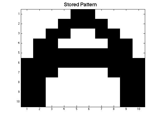
Stored Pattern:

We created a stored pattern on MATLAB by creating a matrix +1’s and -1’s.  Our first pattern is the letter ‘A’, following the examples in Section 12.3 of Giordano and Nakanishi, on a 10×10 matrix.  As mentioned in our earlier posts, each element in the matrix represents a neuron and if the neuron is active it has a value of 1 and if it is inactive, its value is -1. Our ‘A’ pattern is made up of +/-1s where the +1’s represent the pattern and the -1’s represent the background. When these numbers are displayed in the command window, the A pattern is not easy to see, so we use the imagesc command (along with an inverted gray colormap) to better visualize our patterns.

Element Indexing

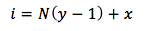
MATLAB indexes the elements in a matrix with two numbers: the first index refers to the row of the matrix, and the second index refers to the column.  For our neural networks, we want to be able to access every element in the array (twice, separately) in order to have every neuron interact with every other neuron.  The easiest way to do this is by using a single number index, i, which runs from 1 to  N².  In our code, we use i and j.  To actually access the elements in our matrices, we have to use the normal double MATLAB indices, which we call call y and x.  The index i can be calculated from the normal y and x indices using equation 12.20 from the text.

In our code, we frequently have two sets of nested for loops, with which we are able to loop through the entire pattern twice, once with the index i and once with the index j.  For this reason, we use the indices y_i,x_i and y_j,x_j.

Interaction Energies J(i,j):

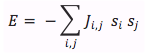
The interaction energy matrix describes the interaction between every neuron with every other neuron. So if we start off with a P_stored matrix of size NxN, then the J matrix for it is going to be size N²x N². In order to determine the values for the J matrix we need to use equation 12.16 from the text,

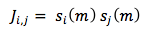
where s_i is the value of neuron i in pattern m, and s_j is the value of neuron j in pattern m.  Thus, the J(i,j) matrix is created by multiplying the values of P_stored(y_i,x_i) with the values of P_stored(y_j,x_j). In order to do this on MATLAB we created two for loops where we held the y(rows) values constant and varied our x (columns) values. By doing this we compare P_stored(1,1) to P_stored(1,2), P_stored(1,3), P_stored(1,4)… Then after finishing with the first row the program goes on to compare P_stored(1,1) with P_stored(2,1), P_stored(2,2)… This continues until P_stored(1,1) is compared with all the other points in the matrix and then it does the same thing for P_stored(1,2), P_stored(1,3), and so on.

Example 1:

Below you will see a P_stored matrix and it’s corresponding J matrix. By using equation 12.20 and the double for loop, you are able to index the values for i and j which allows you to create J(i,j).

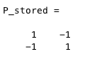  Figure 1  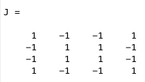                      Figure 2

The interaction energy matrix values will later be used to help determine the amount of energy it takes to activate or inactivate a neuron.

Neural Network Model

After finding our interaction energies, we now have an operational memory for our simple neural network. In order for our neural network to be operational we need to create a pattern within P_stored. In order to do this we created an image of the letter A by manually entering in the 1s to create the letter A. We then created a new matrix called P_in to represent the matrix that we will sweep using the Monte Carlo method. P_in is created by randomly flipping the value of some of the neurons in order to distort our original A pattern. In order to make it easier to visualize, we used the function imagesc to turn our matrix values into an image.

After conducting a Monte Carlo sweep over our distorted A-pattern P_in we should get in return the same pattern as our P_stored matrix. Thus, our neural network remembers being fed the desired pattern we stored earlier. In the figures below, the black squares are represented by +1’s in our matrix and the white squares represent the -1’s.

Figure 3

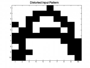 Figure 4 Figure 5

Monte Carlo Method

The method by which the input pattern is changed into the output pattern is the Monte Carlo method.  The essence of this method is to calculate, for each neuron in the input pattern, the effective energy of the entire neural network in its current state using Equation 12.14.

If the total energy of the network with respect to the neuron i is greater than 0, then neuron i’s value is flipped (+1 -> -1, or vice versa).  If the total energy of the neural network with respect to neuron i is less than 0, its value is unchanged.

This process is carried out for every neuron i, so that every neuron is given a chance to flip.  Once every neuron has been checked, one sweep of the Monte Carlo method is complete.

For our current code, we are only using one Monte Carlo sweep, but as we progress forward we will use multiple Monte Carlo sweeps to check if the output pattern is stable, and to see if multiple steps are needed in order to fully recall the stored pattern.

Our full script that includes all the parts discussed above, is attached below.

Brian and Tewa Initial Code for Neural Networks Project

Future Plans

Next, we will begin to characterize the properties of our model.  We will be investigating questions how different P_in is from the stored pattern, the maximum number of patterns that can be stored in a network, and how long pattern recall can take.  The work for this post was done exclusively together as a team, and moving forward we will begin to split up a bit more as we tackle independent questions.  As we do this, we will be splitting up our code into smaller chunks, some of which will be re-defined as functions, for easier interaction.

The first simulation used in this project was for the precession of the perihelion of Mercury. This involves calculation of Mercury’s orbit using the force law as predicted by general relativity:

We can use the above equation to calculate position and velocity; I used a second-order Runge-Kutta Method. Equations shown are the same for x and y:

Once we have the proper position of Mercury we can convert said position to an angle theta. Then, plotting time against theta we can do a linear fit, the slope of which will be our desired rate of precession. A simulated orbit for Mercury, using alpha = .008, appears as shown:

which already shows the precession of the perihelion over time. In the upcoming weeks I need to more closely investigate the rate of this procession.

The second part of the project involves the investigation of Kirkwood Gaps, or the odd behaviour of solar satellites at certain orbital radii which “happen” to coincide with resonances of Jupiter’s orbit. This meant creating a multi-body simulation (I chose 3-body), so as to calculate the position and velocities of our planets (here, Earth and Jupiter), which are then used to calculate the position and velocities of our asteroids. Luckily, the mass of the asteroid is negligible as compared to that of our largest and most impactful orbiting body, Jupiter, and so the effect of the asteroids on Jupiter’s orbit can be ignored. The initial radius and velocity values used for the asteroids are found in Table 4.4 in Giordano and Nakanishi. Again the Runge-Kutta method was used to compute values. The equations used to calculate these values for planets are similar to the Runge-Kutta equations above and are shown by others doing similar celestial mechanics problems. Using this method I plotted first the orbits of Earth and Jupiter, to make sure my simulation worked:

and then plotted the asteroids’ orbits:

The blue orbit above is for the asteroid found around the 2/1 resonance orbit (ratio of axes is 2:1 for Jupiter:asteroid); here is a visual representation of the effect Jupiter can have on other objects, significantly disturbing their orbit. The next step in this program is to add complexity- more asteroids and a better graphical representation of where these orbital radii “gaps” occur.

Matlab Code:

https://docs.google.com/document/d/1hHy4D-B7eWIbknoHlLHJKvlyEtecRhIF7wupYeuFF1s/

https://docs.google.com/document/d/1jOSlib_gAtcADT_Mc0qFi2PA8n1I2nPnxqqOk_0f34w/

This week I worked on the modeling of Mercury’s orbital motion around the Sun. Using the Euler-Chromer Method and the general relativistic force law (see previous post for a more quantitative description) I was able to create a code that shows Mercury’s movement over several orbits. The value for alpha was used at 0.01 (very much greater than the true value) and that the initial conditions used were when , and . 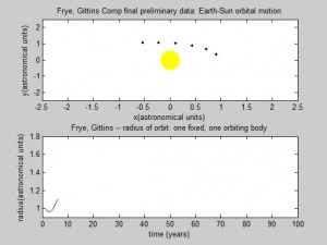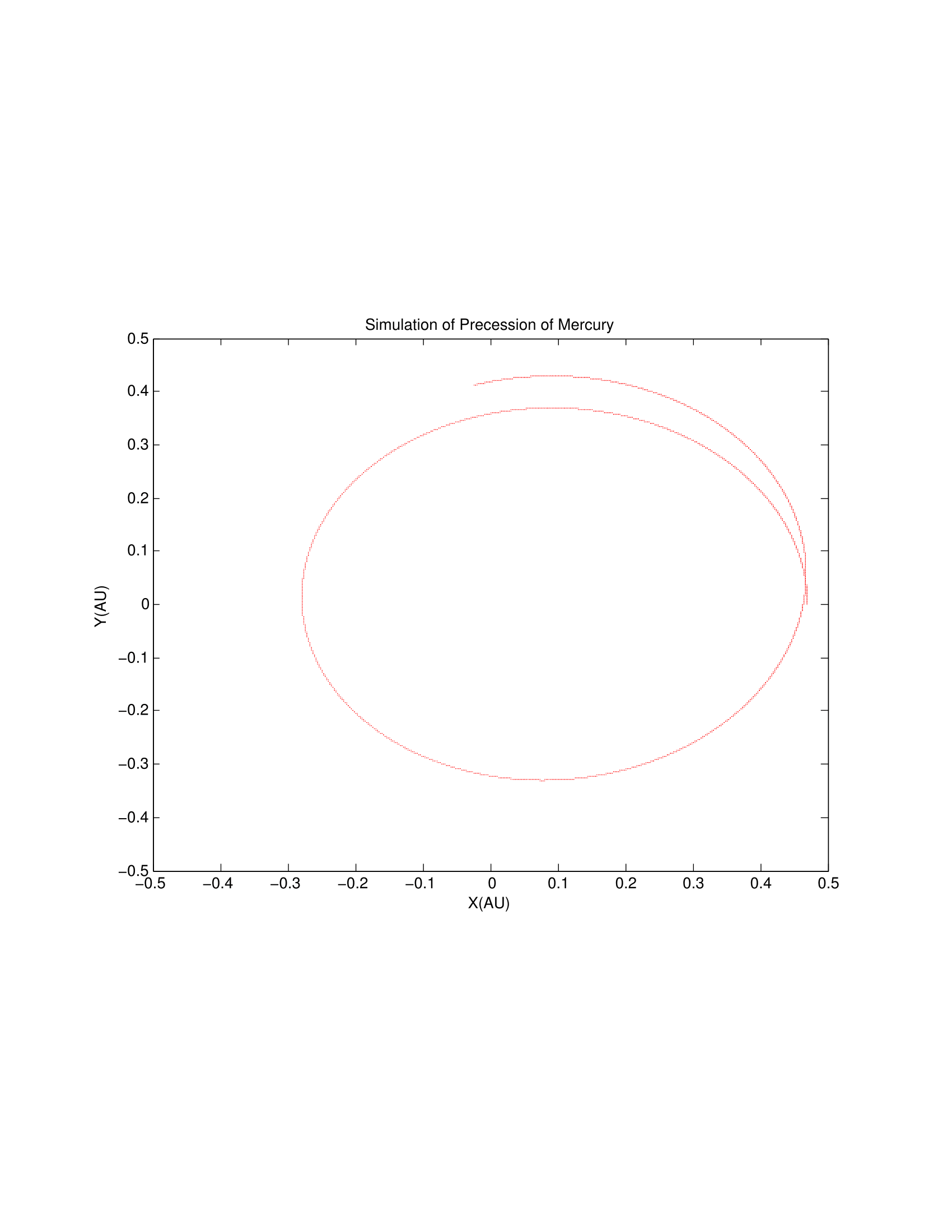It is clear over several orbits that the location of Mercury’s perihelion is changing.

In the following plot, the different positions for the aphelion (chosen for clarity) are clearly shown by lines connecting the origin (or the Sun) to the aphelion.

It is my next goal to determine the amount of degrees by which the orientation of this orbit changes over time. I have run into the issue that Matlab’s acos and asin (arccos and arcsin) functions give imaginary values if their inputs are not with the range of -1<x<1. When this issue is resolved, I will be able to finish deriving the precession rate of Mercury, and will proceed to experimenting with the eccentricity of Mercurian planet orbits and their resulting rates of precession.

Here is a link to my Matlab code: https://docs.google.com/a/vassar.edu/document/d/1fw8L5ZvhqMMVMYltkJH6Ac425KrmnbbDUJs_6GV7aPI/edit?usp=sharing

(Note that equations are rendered in LaTeX which I typed; they simply come through as images, though I include code for documentation.)

My preliminary results were fairly boring, in that I simply executed in MATLAB the guitar simulation central to the first part of chapter 11 of the text. However, this problem was not trivial, and the machinery constructed here will prove critical later in the project.

As background, recall in chapter 6 how the motion of a string was simulated using eq. 6.6:

$latex y(i,n+1)=2[1-r^2]y(i,n)-y(i,n-1)+r^2 [y(i+1,n)+y(i-1,n)]$

where c = speed of wave and r = cΔt/Δx. The force on the bridge (defined here to be the left boundary of the string) can be calculated using eq. 11.4:

$latex F_{\text{bridge}}=T\frac{y(2,n)-y(1,n)}{\Delta x}$

where T is tension, and y(1,n) is the leftmost element on the string at time n (this is a slight modification to the equation in the book, as MATLAB starts indexing at 1, whereas the book’s authors start at 0). For a string plucked at one fifth its length away from the bridge, the following results were obtained after simulating the vibrating string, calculating the force on the bridge with time, and taking the power spectrum of the force using the discrete Fourier transform written for class:

Figure 1: Preliminary data. Bridge power spectrum calculated in MATLAB matches the results in the book very well, indicating that the code used is a good starting point for the rest of the project.

Code used attached here via DropBox (no need to sign up for an account).

Nadav Hendel & Matteo Bjornson

Week One

Our first model, Planets, assumes the sun’s motion due to orbiting planets is negligible and we can keep it fixed at the center of our system. This approximation is a good starting point because the sun is so massive in comparison to any of the planets (Jupiter, the most massive planet, is still no more than 0.1% of the solar mass). The planet motion results from the gravitational force of the sun.  The size of this force is described by

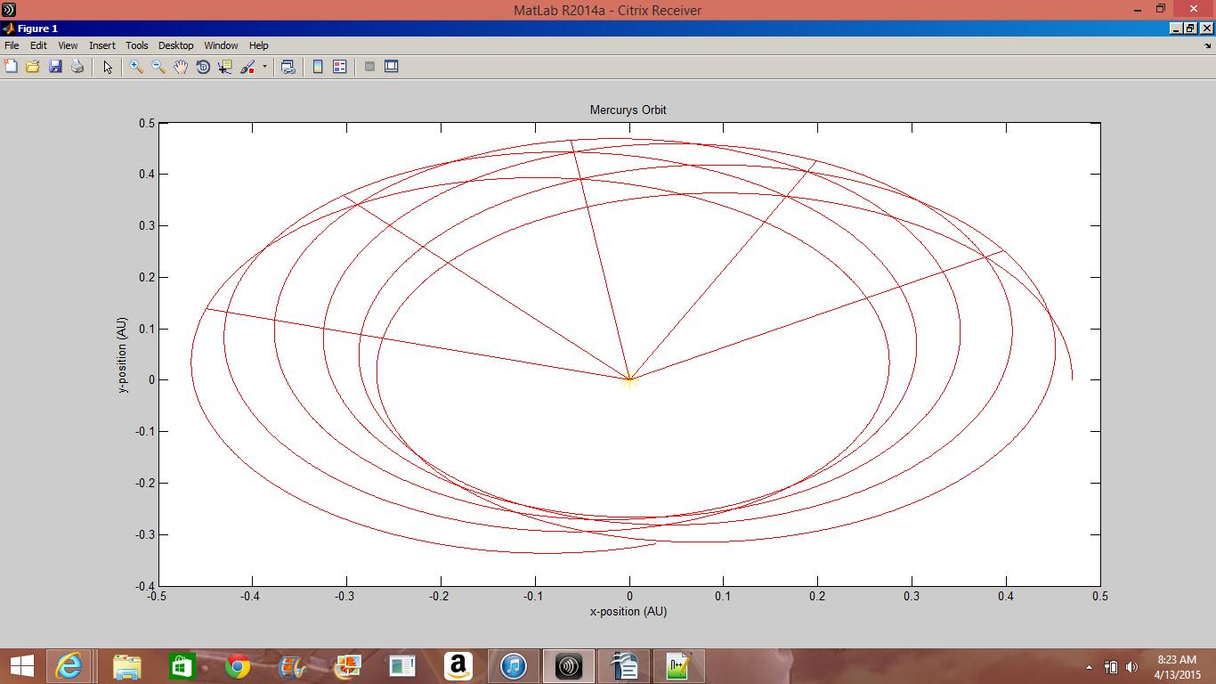
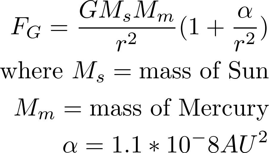
where is the gravitational constant, and are the Solar and planet mass, respectively. is the planet-sun distance.

Due to Newton’s Second Law we know the acceleration of the planet is equal to the force experienced by the planet divided by its mass. This results in a second order differential equation that can be written componentwise as

These can be rewritten as first order differential equations

where and . This program assumes the planet follows uniform circular motion. This is a fairly reasonable approximation to make, as all the planets except Mercury and Pluto have very circular orbits. For example, the eccentricity of Earth’s orbit is under 0.017 [1].  Making this assumption we know that the product is equal to . The average speed of the planet is equal to the distance traveled in one orbit divided by the orbital period, thus . Using units of AU for distance and years for time, the product for Earth (where T=1yr and r=1AU), for example is simply . 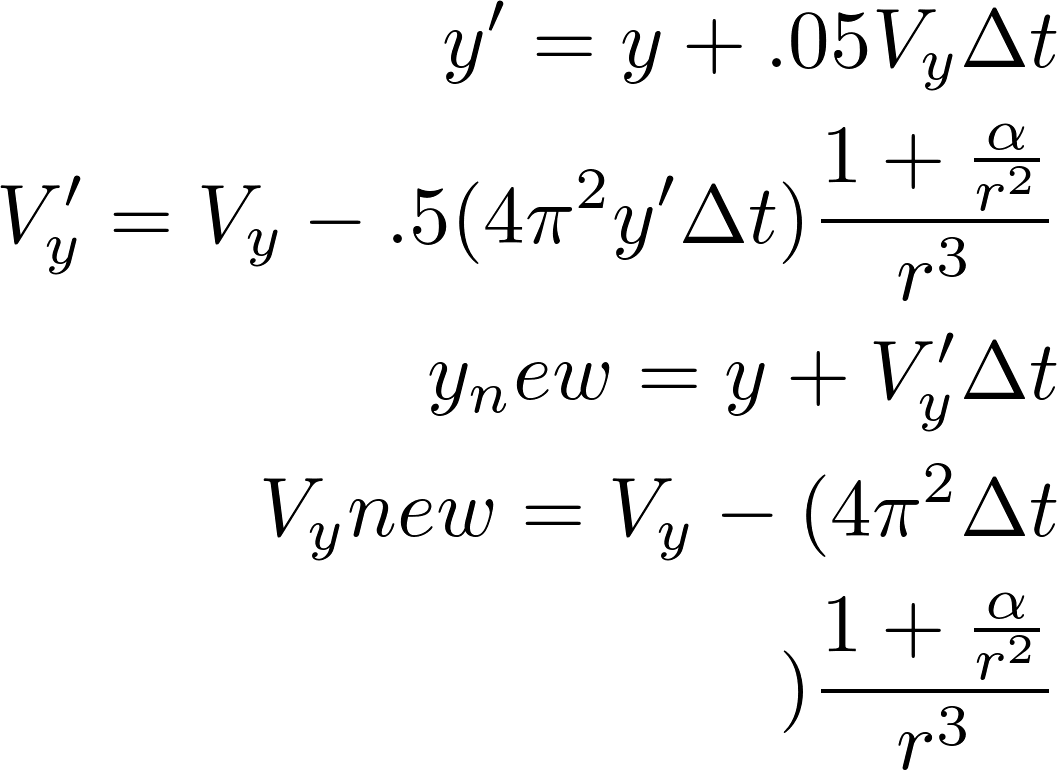Therefore we can rewrite the first order differentials as

The solution to these first order differential equations, x and y, can be approximated using numerical methods. We chose to use the Euler-Cromer Method (Runge-Kutta would work as well), outlined by Giordano, Equations 4.7:

Thus, the only constants necessary to calculate the position of a planet is its orbital period and radius (in this case the semi-major axis). We will be using Astronomical Units (AU) for this section since 1 AU is defined as the average distance between the earth and sun, which has a nearly circular orbit (eccentricity of under 0.017) [1]. Using the Euler-Cromer method, we can create a plot in Planets that traces the earth’s position around the sun due to gravity for a set amount of time.

As long as the average velocity and semi-major axis are known, our program can currently be used to model any other real or hypothetical orbit of a planet around the sun, given the assumption of circular orbits. In fact, we have altered our final subroutine Planets to include the assumed circular orbit for every planet in our solar system excluding Mercury and Pluto. Both of these two planets have eccentricities that are relatively greater than the rest, and are too large to be considered even close to circular. While this is a somewhat subjective judgment made by observation, it seems logical given the relative magnitude of the other planets eccentricities. Given this, the user is prompted at the beginning of the code to pick which planet they wish to observe from the remaining seven.

Now that we have completed a working model for the two-body systems of each planet in our solar system, sans Mercury and Pluto, we wished to do a comparison between computational methods. Since energy must be conserved in our system, similar to the pendulum problems from earlier this semester, we know that difficulties might arise when using the Euler method. To validate this, we wrote another routine implementing Euler instead of Euler Cromer. A comparison of the methods in GIF form is shown below:

Pictured topis the earth’s orbit calculated using the Euler-Cromer method, and bottom is the same code, only run solely using the Euler Method

The radius and velocity of the orbits that we have been modeling are already known to be stable, but we wanted to note what an unstable system using our model might look like. By increasing or reducing the initial velocity, we can observe such a system.

Pictured top is the earth’s orbit calculated using a larger initial velocity by a factor of 2, and bottom is the same orbit using less than ½ original velocity.

Given our goals for week one, we believe we now have a good foundation to expand our Planet routine into a multi-body system. We have become confident with the Euler-Cromer method over the Euler Method, and we have explored the boundaries of our system given different initial conditions. Also, through exploration of chapter four in the Giordano text, we have expanded our understanding of the computational methods used to solve general celestial mechanical problems.

Please click the Matlab Icon to download our Planet routine code

The first simulation we wrote was a simulation for the orbital movement of a planet such as Earth as it orbits the Sun. The orbital motion program was built using the Euler-Cromer method, as specified in the earlier blog post, with new “guesses” for position iterating through a loop for a specified number of calculations.

Although this program is great for visualizing the orbital motion of an object, there were many assumptions made in the creation of the simulation.

The most blatant simplification made was that this is a two-body system. There are of course many more planets in the real solar system, but for the sake of this first simulation, they were ignored. It is not a study of their true motion, but more a simplified circular orbit of a planet (Earth) about the sun. The mass of the Sun and Earth are not even part of the program because they are not significant factors when the mass of the Sun is significantly larger than the mass of the Earth.

We assumed that the sun does not move. Although this is almost true (because Ms>>Me), in reality, the Sun would move in a small orbit that responded to the Earth’s larger motion. Additionally, the Earth would not move in a perfect circular motion but rather in an elliptical direction.

However, this visualization remains a valuable tool for both the conceptualization of an orbital system and also for the further understanding of the Euler-Cromer method. Because it is iterative, and uses the most recent information to continue its guesses, making the approximation relatively accurate.

This is a useful program, but can definitely be more specific and more physically accurate. Our next step should be to try to either add a second planet, or for an extra challenge, adding the moon orbiting our already-orbiting Earth. Additionally, there should be a way for matlab to generate a more visually pleasing result, with a moving planet that leaves a tail behind for us to see the final orbit.

Screenshots of the orbital movement:

We then explored the affect on the orbit if the initial velocity was higher than our original initial velocity. We discovered that by increasing the initial velocity by 10%, the orbit would become elliptical, with the Sun at an off-center focus point. The radius is 1AU at the perihelion, or the fastest moving point, and approximately 1.72 at the aphelion. This is consistent Kepler’s First Law.

The Matlab script:

https://docs.google.com/a/vassar.edu/document/d/1gHvpNnY2pMAh-y2DEihLfF9S7EOxLUb2zZ_FVGl99Qo/edit?usp=sharing

I have a preliminary code for the two dimensional random walk. I think it would be much simpler for me to use a displacement needed to get to a location instead of making it to a location for now. I do not have the data displayed on the figure but it is in the matrices. I also have a preliminary code for Brownian Motion but it is very similar to 2D motion. The largest difference is that it does not follow unit vectors. I would like to see how this could affect displacement. I still need more time to finish up my fits and correct for proper units within those fits but I should be in pretty good shape. I would also like to tinker more with the Brownian Motion code to come up with more interesting visualizations. Comparing pure Brownian motion with my novel 2D walk code is my ideal case. Adding more variables to my 2D walk code will come later since I would still like to compare the differences between random 2D walk and Brownian motion. In order to add more variables, I only need to add more “elseif”‘s to my program.

Here are my preliminary programs:

https://docs.google.com/a/vassar.edu/document/d/1nvyB5giUicIIiCJuKNKTwJagBlepP8J-IOQsMeMgB7Q/edit?usp=sharing