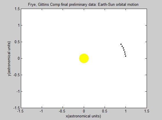
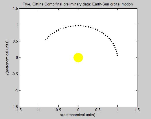
The first simulation we wrote was a simulation for the orbital movement of a planet such as Earth as it orbits the Sun. The orbital motion program was built using the Euler-Cromer method, as specified in the earlier blog post, with new “guesses” for position iterating through a loop for a specified number of calculations.

Although this program is great for visualizing the orbital motion of an object, there were many assumptions made in the creation of the simulation.

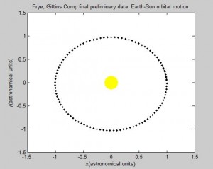
The most blatant simplification made was that this is a two-body system. There are of course many more planets in the real solar system, but for the sake of this first simulation, they were ignored. It is not a study of their true motion, but more a simplified circular orbit of a planet (Earth) about the sun. The mass of the Sun and Earth are not even part of the program because they are not significant factors when the mass of the Sun is significantly larger than the mass of the Earth.

We assumed that the sun does not move. Although this is almost true (because Ms>>Me), in reality, the Sun would move in a small orbit that responded to the Earth’s larger motion. Additionally, the Earth would not move in a perfect circular motion but rather in an elliptical direction.

However, this visualization remains a valuable tool for both the conceptualization of an orbital system and also for the further understanding of the Euler-Cromer method. Because it is iterative, and uses the most recent information to continue its guesses, making the approximation relatively accurate.

This is a useful program, but can definitely be more specific and more physically accurate. Our next step should be to try to either add a second planet, or for an extra challenge, adding the moon orbiting our already-orbiting Earth. Additionally, there should be a way for matlab to generate a more visually pleasing result, with a moving planet that leaves a tail behind for us to see the final orbit.

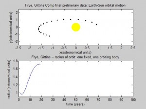
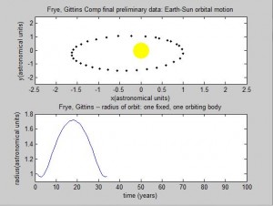
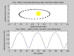
Screenshots of the orbital movement:

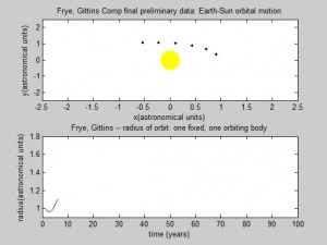
We then explored the affect on the orbit if the initial velocity was higher than our original initial velocity. We discovered that by increasing the initial velocity by 10%, the orbit would become elliptical, with the Sun at an off-center focus point. The radius is 1AU at the perihelion, or the fastest moving point, and approximately 1.72 at the aphelion. This is consistent Kepler’s First Law.

The Matlab script:

https://docs.google.com/a/vassar.edu/document/d/1gHvpNnY2pMAh-y2DEihLfF9S7EOxLUb2zZ_FVGl99Qo/edit?usp=sharing