The first simulation used in this project was for the precession of the perihelion of Mercury. This involves calculation of Mercury’s orbit using the force law as predicted by general relativity:

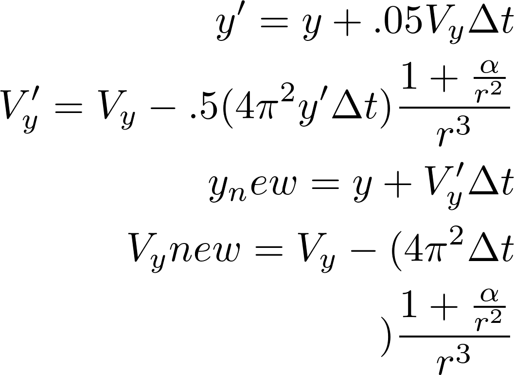
We can use the above equation to calculate position and velocity; I used a second-order Runge-Kutta Method. Equations shown are the same for x and y:

Once we have the proper position of Mercury we can convert said position to an angle theta. Then, plotting time against theta we can do a linear fit, the slope of which will be our desired rate of precession. A simulated orbit for Mercury, using alpha = .008, appears as shown:

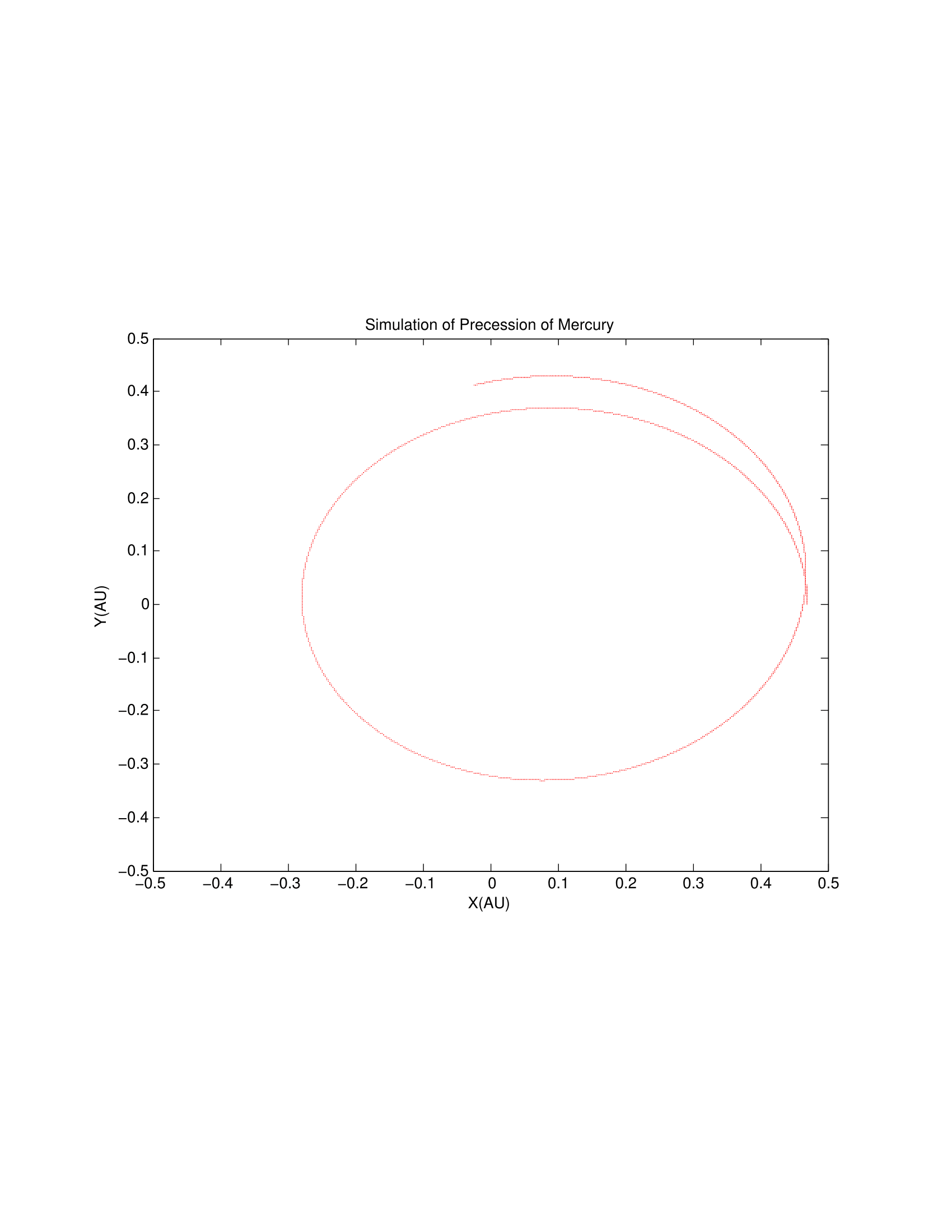
which already shows the precession of the perihelion over time. In the upcoming weeks I need to more closely investigate the rate of this procession.

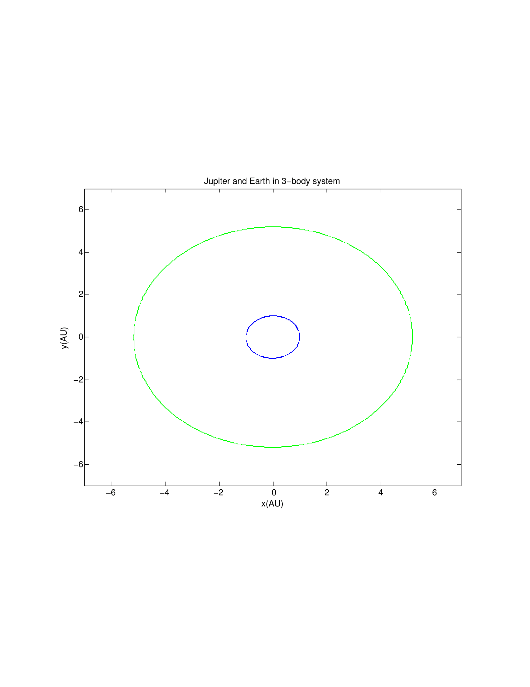
The second part of the project involves the investigation of Kirkwood Gaps, or the odd behaviour of solar satellites at certain orbital radii which “happen” to coincide with resonances of Jupiter’s orbit. This meant creating a multi-body simulation (I chose 3-body), so as to calculate the position and velocities of our planets (here, Earth and Jupiter), which are then used to calculate the position and velocities of our asteroids. Luckily, the mass of the asteroid is negligible as compared to that of our largest and most impactful orbiting body, Jupiter, and so the effect of the asteroids on Jupiter’s orbit can be ignored. The initial radius and velocity values used for the asteroids are found in Table 4.4 in Giordano and Nakanishi. Again the Runge-Kutta method was used to compute values. The equations used to calculate these values for planets are similar to the Runge-Kutta equations above and are shown by others doing similar celestial mechanics problems. Using this method I plotted first the orbits of Earth and Jupiter, to make sure my simulation worked:

and then plotted the asteroids’ orbits:

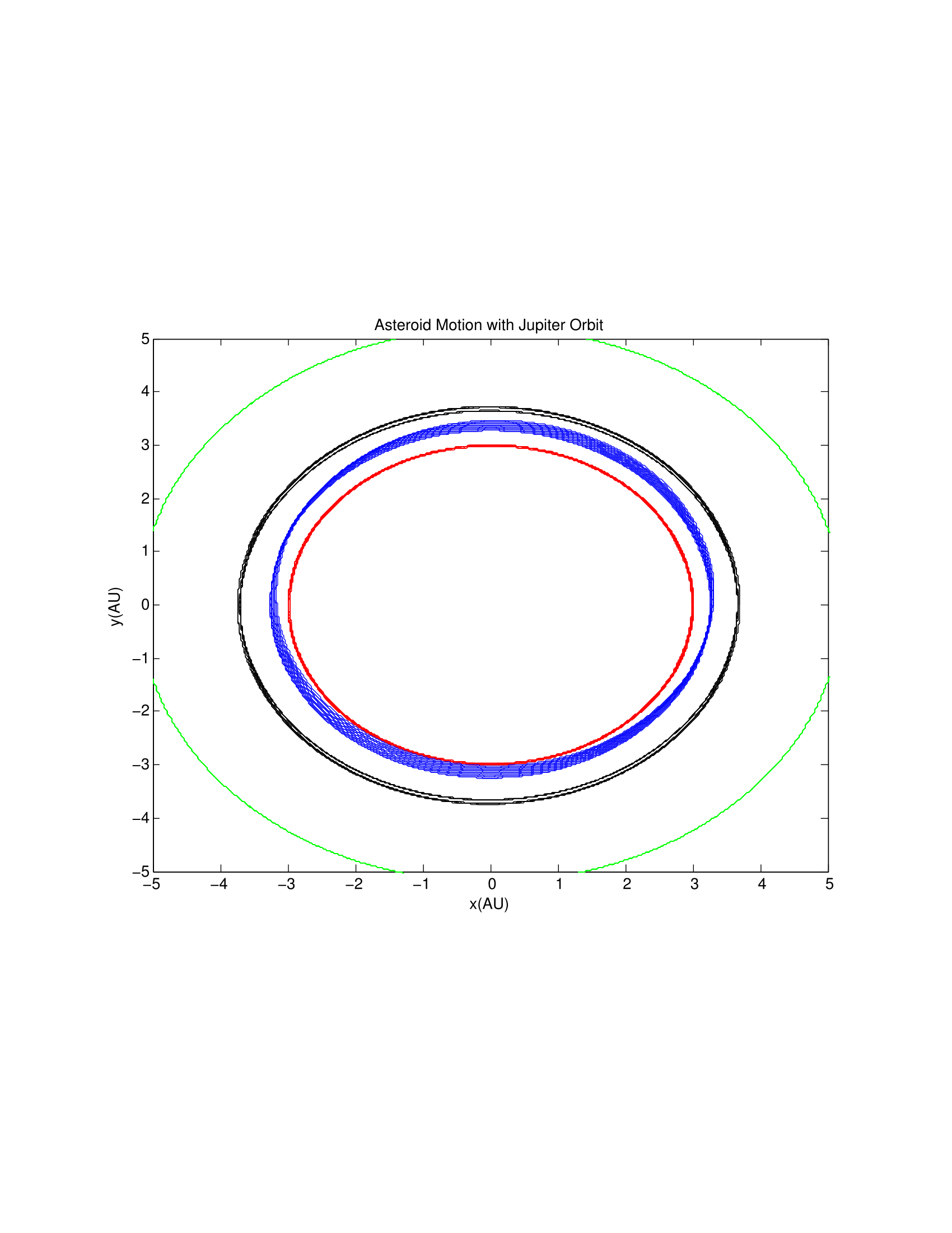
The blue orbit above is for the asteroid found around the 2/1 resonance orbit (ratio of axes is 2:1 for Jupiter:asteroid); here is a visual representation of the effect Jupiter can have on other objects, significantly disturbing their orbit. The next step in this program is to add complexity- more asteroids and a better graphical representation of where these orbital radii “gaps” occur.

Matlab Code:

https://docs.google.com/document/d/1hHy4D-B7eWIbknoHlLHJKvlyEtecRhIF7wupYeuFF1s/

https://docs.google.com/document/d/1jOSlib_gAtcADT_Mc0qFi2PA8n1I2nPnxqqOk_0f34w/