Nadav Hendel & Matteo Bjornson

Week One

Our first model, Planets, assumes the sun’s motion due to orbiting planets is negligible and we can keep it fixed at the center of our system. This approximation is a good starting point because the sun is so massive in comparison to any of the planets (Jupiter, the most massive planet, is still no more than 0.1% of the solar mass). The planet motion results from the gravitational force of the sun.  The size of this force is described by

where is the gravitational constant, and are the Solar and planet mass, respectively. is the planet-sun distance.

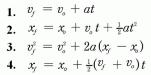
Due to Newton’s Second Law we know the acceleration of the planet is equal to the force experienced by the planet divided by its mass. This results in a second order differential equation that can be written componentwise as

These can be rewritten as first order differential equations

where and . This program assumes the planet follows uniform circular motion. This is a fairly reasonable approximation to make, as all the planets except Mercury and Pluto have very circular orbits. For example, the eccentricity of Earth’s orbit is under 0.017 [1].  Making this assumption we know that the product is equal to . The average speed of the planet is equal to the distance traveled in one orbit divided by the orbital period, thus . Using units of AU for distance and years for time, the product for Earth (where T=1yr and r=1AU), for example is simply . Therefore we can rewrite the first order differentials as

The solution to these first order differential equations, x and y, can be approximated using numerical methods. We chose to use the Euler-Cromer Method (Runge-Kutta would work as well), outlined by Giordano, Equations 4.7:

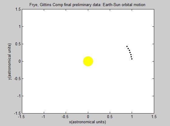
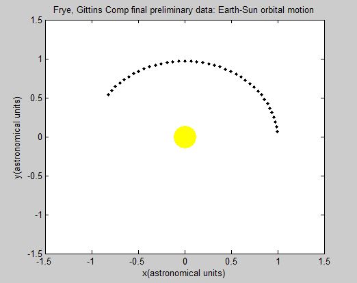
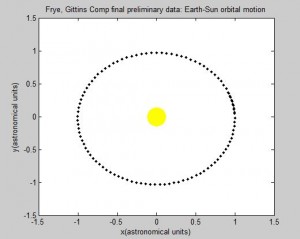
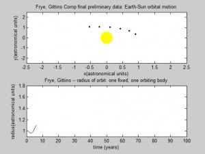
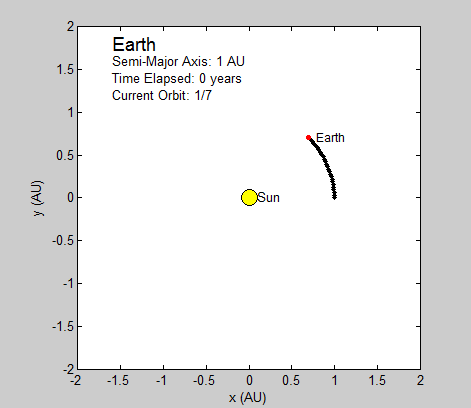
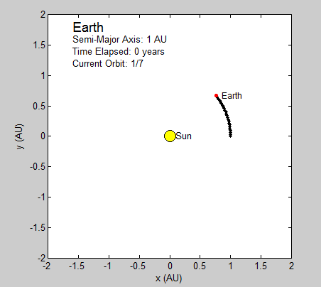
Thus, the only constants necessary to calculate the position of a planet is its orbital period and radius (in this case the semi-major axis). We will be using Astronomical Units (AU) for this section since 1 AU is defined as the average distance between the earth and sun, which has a nearly circular orbit (eccentricity of under 0.017) [1]. Using the Euler-Cromer method, we can create a plot in Planets that traces the earth’s position around the sun due to gravity for a set amount of time.

As long as the average velocity and semi-major axis are known, our program can currently be used to model any other real or hypothetical orbit of a planet around the sun, given the assumption of circular orbits. In fact, we have altered our final subroutine Planets to include the assumed circular orbit for every planet in our solar system excluding Mercury and Pluto. Both of these two planets have eccentricities that are relatively greater than the rest, and are too large to be considered even close to circular. While this is a somewhat subjective judgment made by observation, it seems logical given the relative magnitude of the other planets eccentricities. Given this, the user is prompted at the beginning of the code to pick which planet they wish to observe from the remaining seven.

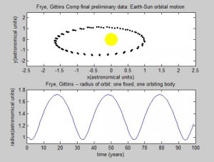
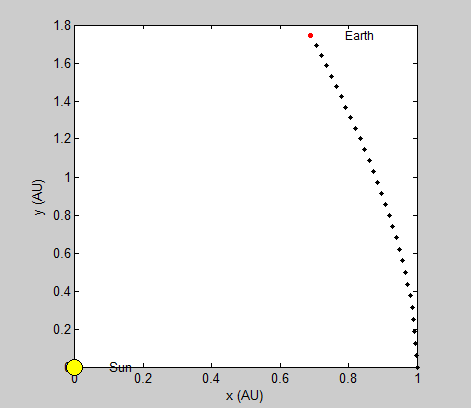
Now that we have completed a working model for the two-body systems of each planet in our solar system, sans Mercury and Pluto, we wished to do a comparison between computational methods. Since energy must be conserved in our system, similar to the pendulum problems from earlier this semester, we know that difficulties might arise when using the Euler method. To validate this, we wrote another routine implementing Euler instead of Euler Cromer. A comparison of the methods in GIF form is shown below:

Pictured topis the earth’s orbit calculated using the Euler-Cromer method, and bottom is the same code, only run solely using the Euler Method

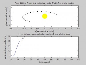
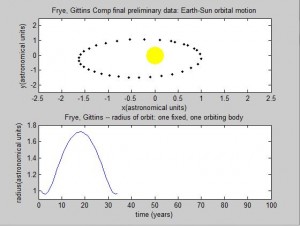
The radius and velocity of the orbits that we have been modeling are already known to be stable, but we wanted to note what an unstable system using our model might look like. By increasing or reducing the initial velocity, we can observe such a system.

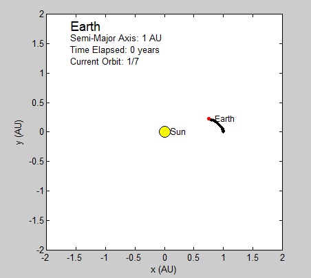
Pictured top is the earth’s orbit calculated using a larger initial velocity by a factor of 2, and bottom is the same orbit using less than ½ original velocity.

Given our goals for week one, we believe we now have a good foundation to expand our Planet routine into a multi-body system. We have become confident with the Euler-Cromer method over the Euler Method, and we have explored the boundaries of our system given different initial conditions. Also, through exploration of chapter four in the Giordano text, we have expanded our understanding of the computational methods used to solve general celestial mechanical problems.

Please click the Matlab Icon to download our Planet routine code

The first simulation we wrote was a simulation for the orbital movement of a planet such as Earth as it orbits the Sun. The orbital motion program was built using the Euler-Cromer method, as specified in the earlier blog post, with new “guesses” for position iterating through a loop for a specified number of calculations.

Although this program is great for visualizing the orbital motion of an object, there were many assumptions made in the creation of the simulation.

The most blatant simplification made was that this is a two-body system. There are of course many more planets in the real solar system, but for the sake of this first simulation, they were ignored. It is not a study of their true motion, but more a simplified circular orbit of a planet (Earth) about the sun. The mass of the Sun and Earth are not even part of the program because they are not significant factors when the mass of the Sun is significantly larger than the mass of the Earth.

We assumed that the sun does not move. Although this is almost true (because Ms>>Me), in reality, the Sun would move in a small orbit that responded to the Earth’s larger motion. Additionally, the Earth would not move in a perfect circular motion but rather in an elliptical direction.

However, this visualization remains a valuable tool for both the conceptualization of an orbital system and also for the further understanding of the Euler-Cromer method. Because it is iterative, and uses the most recent information to continue its guesses, making the approximation relatively accurate.

This is a useful program, but can definitely be more specific and more physically accurate. Our next step should be to try to either add a second planet, or for an extra challenge, adding the moon orbiting our already-orbiting Earth. Additionally, there should be a way for matlab to generate a more visually pleasing result, with a moving planet that leaves a tail behind for us to see the final orbit.

Screenshots of the orbital movement:

We then explored the affect on the orbit if the initial velocity was higher than our original initial velocity. We discovered that by increasing the initial velocity by 10%, the orbit would become elliptical, with the Sun at an off-center focus point. The radius is 1AU at the perihelion, or the fastest moving point, and approximately 1.72 at the aphelion. This is consistent Kepler’s First Law.

The Matlab script:

https://docs.google.com/a/vassar.edu/document/d/1gHvpNnY2pMAh-y2DEihLfF9S7EOxLUb2zZ_FVGl99Qo/edit?usp=sharing

I have a preliminary code for the two dimensional random walk. I think it would be much simpler for me to use a displacement needed to get to a location instead of making it to a location for now. I do not have the data displayed on the figure but it is in the matrices. I also have a preliminary code for Brownian Motion but it is very similar to 2D motion. The largest difference is that it does not follow unit vectors. I would like to see how this could affect displacement. I still need more time to finish up my fits and correct for proper units within those fits but I should be in pretty good shape. I would also like to tinker more with the Brownian Motion code to come up with more interesting visualizations. Comparing pure Brownian motion with my novel 2D walk code is my ideal case. Adding more variables to my 2D walk code will come later since I would still like to compare the differences between random 2D walk and Brownian motion. In order to add more variables, I only need to add more “elseif”‘s to my program.

Here are my preliminary programs:

https://docs.google.com/a/vassar.edu/document/d/1nvyB5giUicIIiCJuKNKTwJagBlepP8J-IOQsMeMgB7Q/edit?usp=sharing

The primary goal of this week was to further our understanding of the Monte Carlo method works. To do this we researched basic modes of how the Monte Carlo method operates. The Monte Carlo method relies on the repeated random sampling to obtain numerical results. We decided to demonstrate how this method can be used to illustrate the distribution of numbers of two dice rolled for an arbitrarily number of times. 

As expected, 7 is rolled the most amount of times.

One of the most basic Monte Carlo methods is the calculation of the value of pi. Look at the following picture, in which a black unit circle is inscribed into a white square: 

We know that the ratio of the area of the circle to that of the square is pi/4. If you need to prove this to yourself, simply divide the area of a circle by that of a square whose sides are twice the length of the circle’s radius. Now, imagine that you dropped a series of evenly and randomly distributed darts across the image. If you counted them, the number of darts within the circle should be about pi/4 times the amount of total darts dropped. It is much easier to simply count these darts than to try any other mathematical measurement. The following code allows us to simulate this scenario by randomly selecting coordinates within the image above. If the randomly selected coordinate has a value of 0, it is black and thus it is counted as having landed in the circle. Most of the trials yield a value of about 3.09, relatively close to pi. We believe that it is off because MatLab is not able to perfectly represent a circle as values in an array.

We then began to research basic option trading techniques. Option trading is a large field in the world of finance and uses computer simulations to traders. To start it was necessary to understand what an option is. The definition from Aswath Damodaran gives a simple, and concise answer: “An option provides the holder with the right to buy or sell a specified quantity of an underlying asset at a fixed price (called a strike price or an exercise price) at or before the expiration date of the option.” To fully understand this definition, it is critical to know that an underlying asset simply means a stock or a portfolio for our purposes.

Option trading typically uses binomial trees or the Black-Scholes method. The Black-Scholes method was published in 1973 and won the Nobel Prize in Economics in 1997, is a way of finding the end price of underlying asset given specified parameters. These parameters include: the strike price, K, the asset price, S, the volatility given by the symbol $\sigma$, the risk free interest rate, r, and the time until maturity T. The Black-Scholes model can be used for two different types of options, a put option and a call option. A call option provides the holder the right to buy the underlying asset at the specified strike price until the maturity date. Conversely, a put option gives the holder the right to sell an underlying asset at the strike price at any point until the maturity date.

For a less technical definition, lets say stock A is being traded for 10 dollars and you can purchase the call option for 2 dollars giving you the right to sell stock A for 10 dollars (the strike price). You believe that stock A will go up to fifteen dollars in a month, so you spend 200 dollars on 100 shares. Fortunately stock A has gone up to 20 dollars, so now you invoke your right to purchase 100 shares at 10 dollars each and then immediately sell stock A. This gives you a profit of 10 dollars a share giving a net profit of 800 dollars because we must take into account the 200 dollars you spent on the call option.  The Black-Scholes model is below:

(1)  

where

(2)  

and

(3)  

$N(d_1)$ is the standard normal distribution of $d_1$ and $N(d_2)$ is the standard normal distribution of $d_2$.

In our code we found the call option for a European option because it is slightly easier to code. For the parameters: $\sigma$ = .3, K=4, S=2, T=3, and r=.4 we get the call option price from the Black-Scholes model is .86415 and from the Monte Carlo method we get .86509. The Monte Carlo method provides a powerful way to check that our solution to the Black-Scholes model is correct. In our case we use an extremely large amount of random numbers. To check our example we encourage you to run our code, which can be downloaded at the link provided at the bottom of the page. Our code runs for the European Call Option and can be checked against: http://www.erieri.com/blackscholes.

A more advanced Monte Carlo method is used to solve an ising model that represents the spin states of electrons in a magnetic material. Here, we have defined the “isinggrid” to represent a system of interdependent spins. These spins naturally tend to align themselves in the same direction, and thus we have started with a ferromagnetic system in which all spins are aligned. We then simulate stochastic changes in the system that occur because of energy added by the temperature in a heat bath. As temperature rises, the greater there is that one of the spins will orient itself in a way that requires adding energy to the system. This is because the extra heat from the increased temperature supplies extra energy. We have also accounted for the spins at the edges of the grid by applying periodic boundary conditions that allow even spins on the edge to interact with four neighbors instead of two or three. We iterate through 11 temperatures in this example, calculating the overall magnetization for each one. This magnetization, M, is the average magnetization calculated 5000 times by the stochastic Monte Carlo process. If a spin flip results in a decrease in energy of the system, it occurs. If it increases the energy, the program generates a random number and then compares it to a parameter set by the temperature. Below is the average magnetization for each temperature that we tried:

As we can see, there is a very sharp drop off in Magnetization upon reaching a certain temperature, which we will calculate the exact value of by next week. This is a good step in our project, as it is important for us to get used to working with stochastic and semi-stochastic systems. Our financial models will involve similar sorts of ideas.

Link to our code: https://drive.google.com/folderview?id=0B01Mp3IqoCvhflF5azV4bHY2V0c3Vks0VXVyQkIxcnR4RmFaNDhVWEQtZGZSR2t6V2VWOHc&usp=sharing

New References:

1. The Black and Scholes Model: http://bradley.bradley.edu/~arr/bsm/pg04.html

2. Aswath Damodaran http://people.stern.nyu.edu/adamodar/pdfiles/option.pdf

3. Bruce Mizrach  http://snde.rutgers.edu/pubs/[42]-2010_Handbook.pdf

Sushant Mahat and Mohammed Abdelaziz

We created two functions to simulate the movement of dilute gas molecules in a container.

The first function initiates a grid of equally spaced points on which to initially place each particle. The function gives them random velocities and perturbs their initial position slightly from the equally spaced grid points.

The second function is a routine that updates the position of each particle at each time step. It determines the next position of each particle by determining the force acting on it due to all other particles in the box, based on the Lennard-Jones potential. The Lennard-Jones potential leads to a force that is large and repulsive at short distances, and attractive at larger distances. The repulsive force has been problematic, because two particles that encounter each other in the box get repelled at very large speeds, producing isolated points like those seen in our results below. If we can solve this issue, the results should be much more coherent.

Additionally, the simulation uses periodic boundary conditions, which we successfully implemented. A particle that “exits” one side of the box must return through the other side at the same velocity. The force calculations reflected this; two distances could be used to calculate the force: one that is between two points within the box, and another that takes into account the periodic boundary conditions. The shorter distance of the two was used to calculate each force.

We ran a calculation of 25 particles in a 10×10 box and obtained these results:

Once again, fixing the exponentially increasing forces is our top priority at this point; once we do so, we will be able to accurately calculate speed and velocity distributions of the particles in the box.

The two functions are attached as .pdf files.

Function 1: TheInitiator

Function 2: TheUpdater

A script was used to initialize variables, run the two functions, and plot the results.

EDIT (4/16/15)
The original *.m files have been uploaded and can be found here.

1. Introduction

The human body is an elastic and versatile model.  It can move muscles individually or in a systematic way in an instant. For our project, we are interested in exploring realistic projectile motion and human acceleration as it pertains to the human body.  While we often assume air resistance and spin to be negligible in Introductory Mechanics, as a way of simplifying our calculations, it is impossible to ignore their effects in competitive events like the long jump.  The additional drag force caused by a single misplaced limb can lead to a loss of centimeters on a jump.  This difference may indeed be negligible in the context of an Introductory Mechanics problem, but is everything to an athlete competing for medals and sponsorship.  For our project, we want to explore the effects of proper body position on the traveled distance in the long jump, in addition to exploring the negative effects of improper position.

2. Project Details

In order to do this, we believe we will need to devise a way of modeling the human body as a 3-dimensional object inside a larger 3-dimensional array representing space.  If we find it necessary later on, we can make the body as low profile as possible by modeling it as a stick figure.  We intend to impart initial conditions onto the object using the “Previous, Current, Next” template we have been using in our homework, to give the body an initial x and y velocity.  The experimentation will occur in the middle of the jump, where we will change the position of various limbs of the body (possibly through matrix multiplication, as is done in computer animation), and compare the results on the final jump distance.  Changing body position will both change the surface area profile of the body, changing the drag force, and change the body’s center of mass which may lead to spin in the face of wind.  We will draw examples of proper and improper form from the literature produced by top track and field coaches so that our program will be grounded in reality and have some practical value.

2. Motivation for Project

Track and Field and athletics in general have been major parts of both of our lives as, between the two of us, we have participated in basketball, volleyball, cross country, track and field, and swimming at a Varsity level.  Also, both of us have considered careers in the Health & Fitness Industry in the past, and are still interested in ongoing developments in the field. We are both interested in the underlying mechanisms that go into making the simplest, and most human tasks, such as walking, running, and jumping, as efficient as possible.  We also both competitive people and have spent years fussing over minute details to give us the smallest competitive advantage.  We are excited to see what we can accomplish now with our improved knowledge of physics and the powerful software at our disposal.

References (will add more at a later time)

Giordano, Nicholas J., and Hisao Nakanishi. “Chapter 2: Realistic Projectile Motion.” Computational Physics. 2nd ed. Upper Saddle River, NJ: Pearson/Prentice Hall, 2006. Print.

Kinematic Equations

Projectile/Range Equations

Timeline (subject to change depending on our work efficiency):

Week 1: The setup. Establishing the arrays, the initial variables and conditions.

Week 2: Run simple trial with one-dimensional object in two-dimensional space with air resistance.  Then second trial with a mass-less two dimensional object in 3-dimensional space.

Week 3: Two test trials with three-dimensional object in three-dimensional space, each with different body position.

Week 4: All trials complete, finalizing the written report and conclusion.

Goals and Sources

The goal of this project is to investigate some simple models of neural networks and memory, which are extensively used in cognitive science and related disciplines to model certain aspects of human brains.  Our project will follow Section 12.3 of Computational Physics by Giordano and Nakanishi, which draws on the Ising and Monte Carlo methods presented in Chapter 8.  This project will be attempting to investigate how to create this type of neural network model, how well it retrieves stored patterns depending on differing input patterns, how many patterns can be stored (and why there is a limit), how well the system functions when parts of the memory are damaged, and how the system learns new patterns.

Background

Chapter 8 introduces the Ising model, which is used to model magnetic substances and phase transitions with temperature changes.  The basics of this model are an array of spins, which are allowed only two orientations: up (+) or down (-).  These spins are connected to their neighbors so that they influence each other; when a negative spin is surrounded by positive ones, the flipping of the negative one to positive represents a reduction of energy.  The Monte Carlo method is used to search through the array, deciding if each spin should be flipped or not, according to its interactions with the surrounding spins, so that the energy of the system tends towards its minimum value.

+ + +           + + +

+  – +    →   + + +

+ + +           + + +

Using a 2-D array of completely interconnected Ising spins, a group of neurons can be modeled and investigated.  These neurons are very simplified, so that they are in only two possible states, firing (+) or not firing (-).  Patterns can be stored in these neural networks by formatting the connections between spins so that stored patterns correspond to energy minima compared to random patterns.  This is accomplished with Equation 12.18

where J_i,j is the connection array (which stores all the connection weights between the neuron spins), M is the total number of stored patterns, s_i (m) and s_j (m) are the configurations of spin i and j in stored pattern m.

Project Timeline

Week 1 (4/6 – 4/12)

We will begin by creating an Ising magnet program and learning the Monte Carlo method, following Chapter 8 and relevant examples closely.  This will set us up to be able to implement these tools on our neural network models later on.

Week 2 (4/13 – 4/19)

Next, we will create a simplified Neural Network, using symmetric connections and storing relatively few patterns, and test this network so that we are sure it functions as it should.  The beginning parts of Section 12.3 will be followed closely here.  In this process, we will figure out most of our code, in terms of creating neural networks, how the neurons are indexed, how to create patterns easily using for loops, how to store these patterns using Equation 12.18, etc.

Week 3 (4/20 – 4/26)

Here we will begin splitting up the topics for further investigation.  Routes of investigation include

a. How far away initial inputs can be from stored patterns while maintaining successful                     recall.

b. How many patterns can be stored in the neural network.  The book discusses the                           maximums associated with this type of neural network, but we will investigate why this                 limit exists, as well as what kinds of behaviors change around this limit.

c. How long (how many Monte Carlo iterations) recall of stored patterns takes.

Tewa will take charge of a and c.

Brian will focus on section b.

Week 4 (4/27 – 5/3)

We will continue to work on the investigations from week 3, and if we have time, we will progress to more complicated neural networks.  Some complications we can introduce are larger networks (and how the recall times might change), asymmetrically connected neurons (a more complicated weight connection matrix), and how further learning impacts the neural networks.

Week 5 (5/4 – 5/10)

We will continue any investigations we have left during this week, and begin writing up our results for final blog posts and presentations.

Week 6 (5/11 – 5/13)

We will finish up our blog posts and presentations, and present our results to the class.

An acoustic plane wave is defined much as you’d expect: as a “plane” of sound energy traversing a medium. When this wave encounters an object, there are several possibile outcomes:

1) Diffraction–the sound is “bent” around the object and its path is therefore altered;
2) Scattering–the sound is reflected off of the object and its path is thus altered;
3) Refraction–the sound passes through the object and its path is therefore altered due to a change in medium.

In this project I shall consider only diffraction and scattering, as the “object” I have chosen is a perfectly rigid, acoustically non-transparent sphere (i.e. sound cannot pass through it). In practice, it is seen that diffraction occurs for high wavelength (low frequency) sound only, and as frequency increases, scattering becomes the dominant phenomenon.

Like any wave, there is a wave equation dictating the propagation of an acoustic wave. Its solution is, however, quite complicated (especially in the presence of objects/barriers), and although analytical solutions exist for diffraction and scattering on a sphere, its components, which require complex functions such as Spherical Bessel and Hankel functions and their derivatives, whose values cannot be precisely (analytically) determined using computational methods, and which therefore must be approximated much like we approximated the solutions to differential equations using the Euler, Runge-Kutta, or similar methods.

For the sake of illustration the acoustic wave equation in three dimensions is:

Notice that this is a 2nd order differential equation the likes of which we have handled in class.

The layout of the project is this (in order of importance):
1) to use the acoustic wave equation to numerically solve the problem of diffraction (low frequencies) and scattering (high frequencies) of the wave on the surface of a rigid sphere;
2) to compare this result to the analytical results available;
3) to provide a visual or graphical representation of the phenomena;
4) to discuss error propagation in numerical method and the method by which the Spherical Bessel and Hankel functions described earlier are approximated;
5) to, if possible, discuss the spherical harmonic decomposition of sound on the surface of the sphere, which provides a rigorous basis for accurately modeling the sound up to a certain frequency.

This last point also requires the evaluation of integrals (in a way analogous to that of Fourier Transforms in 2D), which by the nature of computation are impossible to solve perfectly using numerical methods, but must be approximated as sums. If I am able to include this last point, I will also discuss the method of approximating the integrals.